Tracking an Oscillator

This example continues the Channel Memory simulation demonstration.

A two-operator problem is solved over a network with channel memory, parameterized by a forgetting factor \(\alpha>0\)

\[\begin{split}\begin{align*} z^1_k &= u_k^1 - \alpha z^1_{k-1}, & y_k^1 &= w_k^1 - \alpha y_{k-1}^1, \\ z^2_k &= u_k^2, & y_k^2 &= w_k^2. \end{align*}\end{split}\]

An \(\alpha\)-dependent controller

\[\begin{split} \mat{c}{x_{k+1}^c \hl u_k^1 \\ u_k^2} = \mat{c|cc}{I & -\gamma \lambda & \frac{ -\gamma \lambda}{\alpha+1} \hl (1+\alpha) I & 0 & 0 \\ I & -\gamma I & -\frac{ -\gamma }{\alpha+1} I } \mat{c}{x_{k}^c \hl y_k^1 \\ y_k^2}\end{split}\]

is used to solve the problem with values of \(\gamma = 0.4, \lambda = 0.2\). The operator \(F_1\) is the subdifferential of a function in \(S_{1, 5}\). The operator \(F_2\) is the subdifferential of a function in \(S_{0, \infty}\).

Figure 1 plots Analysis-computed upper-bounds on \(\rho\) as the forgetting factor \(\alpha\) increases. The same order is used for each operator. \(\rho=2\) is used as an upper bound in bisection: a rate of \(\rho<2\) is certified as a worst-case bound.

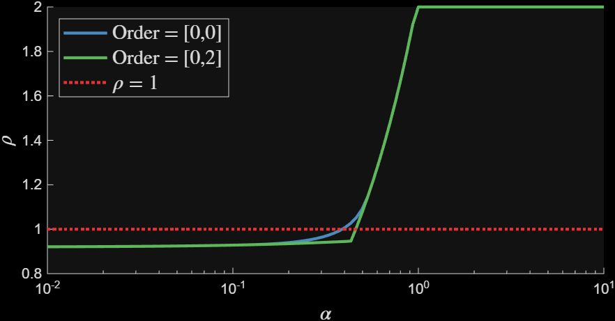
Figure 1: Convergence rate v.s. forgetting factor

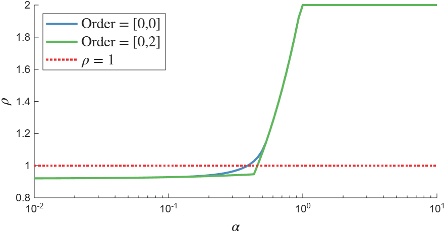
Figure 1: Convergence rate v.s. forgetting factor

Code for Channel Memory sweep analysis

%pose the operator class
m = 1; L = 5;
op1 = op_sml(m, L);

op2 = op_pcc();
ops = {op1, op2};


%use a transfer function representation 
%to model the channel memory
z = tf('z', 1);

%sweep over alpha and order
Nalpha = 100;
alpha_list = logspace(-2, 1, Nalpha);
orderlist = {0, [1, 0], [0, 1], [1, 1], [2, 0], [0,2]};
Norder = length(orderlist);
rho_list = zeros(Nalpha, Norder);


parfor i = 1:Nalpha
    alpha = alpha_list(i);
    ascale = (2*(alpha+1));
    
    %form the channel memory network
    P = [0, 0, z/(z+alpha), 0;
        0 , 0, 0, 1;
        z/(z+alpha), 0, 0, 0;
        0, 1, 0, 0];
    
    network = genplant(P);
    network.nw = 2; network.nu = 2;
    network.nz = 2; network.ny = 2;

    %create the controller
    gamma = 0.4;
    lambda = 0.2;

    K = ss([1], [-gamma*lambda, -gamma*lambda/(alpha+1)], ...
        [1+alpha; 1], [0, 0; -gamma, -gamma/(alpha+1)],1);
    
    sys = opt_system(ops, network, K);
    
    %solve Analysis at each order
    man = opt_analysis(sys);    
    for j = 1:Norder
        order = {orderlist{j}, orderlist{j}};
        sol = man.bisect(order);
        rho_list(i, j) = sol.rho;
    end
       
end