

Proximal Heavy Ball#
The Proximal Heavy Ball algorithm is a scheme to solve composite optimization problems \(\min_\beta f(\beta) + g(\beta)\) (Sec. 2.5.3. [1]).
The description of the Proximal Heavy Ball algorithm is with parameters \(\gamma, \lambda > 0\) is
Analysis is performed to upper-bound the convergence worst-case rate \(\rho\) for parameter choices \(\gamma = \frac{2}{m+L}\) and \(\lambda = 0.65\).
The operators \(\nabla f\) and \(\partial g\) are Analyzed each with orders [3, 0] or [3, 1].
The parameter \(L\) swept in the range \([1, 500]\) with fixed \(m=1\). \(f\) is restricted to general functions in \(S_{m, L}\) or to quadratics in \(S_{m, L}\), and \(g\) is a member of \(S_{0, \infty}\).
Figure 1 plots the computed \(\rho\) upper bounds at each order and operator class. The worst-case convergence rate \(\rho\) is reduced by restricting to quadratic \(f\) as compared to general \(f \in S_{m, L}\).
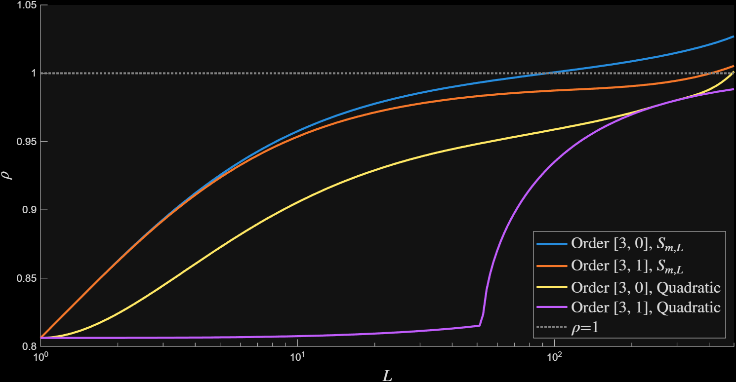
Figure 1: Estimates of the Proximal Heavy Ball convergence rate#
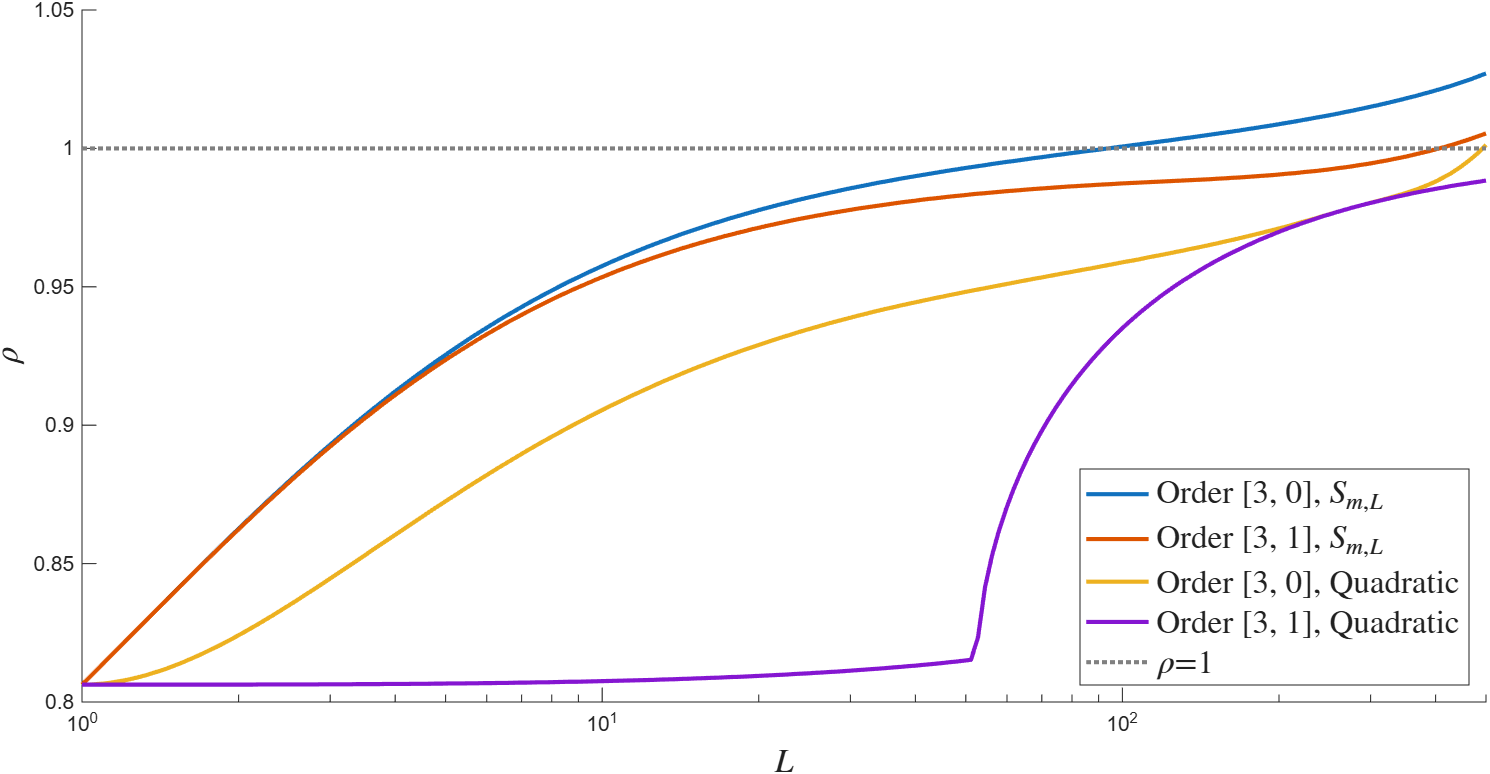
Figure 1: Estimates of the Proximal Heavy Ball convergence rate#
 1%parameters of the sweep
 2NL = 200;
 3Llist = logspace(0, log10(500), NL);
 4
 5orderlist = {
 6    {[3, 0], [3, 0]};
 7    {[3, 1], [3, 1]}
 8    };
 9Norder = length(orderlist);
10
11
12%analysis of proximal heavy ball algorithm
13parfor i = 1:NL
14    m= 1;
15    L = Llist(i);
16
17
18    %different operator classes for \nabla f
19    op1_sml = op_sml(m, L);
20    op1_quad = op_quad(m, L);
21
22    %indicator function for \partial g
23    op2 = op_sml(0, inf, 1);
24
25    %proximal heavy ball
26    gamma = 2/(m+L);
27    lambda = 0.65;
28
29    A = [1+lambda, -lambda; 1, 0];
30    B = [-gamma, -gamma; 0 , 0];
31    C = [1, 0; 1+lambda, -lambda];
32    D = [0, 0; -gamma, -gamma];
33
34    sK = ss(A, B, C, D, 1);
35
36    %form the system
37    sys_sml = opt_system({op1_sml,  op2}, [], sK);
38    sys_quad = opt_system({op1_quad, op2}, [], sK);
39
40    %pose and solve the problem
41    man_sml = opt_analysis(sys_sml);
42    man_quad = opt_analysis(sys_quad);
43
44    for j = 1:Norder
45        sol_sml = man_sml.bisect(orderlist{j});
46        rho_sml(i, j) = sol_sml.rho;
47
48        sol_quad = man_quad.bisect(orderlist{j});
49        rho_quad(i, j) = sol_quad.rho;
50    end
51
52end
53
54%% plot the result
55figure(4)
56clf
57hold on
58plot(Llist, rho_sml, 'linewidth', 2)
59plot(Llist, rho_quad, 'linewidth', 2)
60
61plot([Llist(1), Llist(end)], [1, 1], ':', 'linewidth', 2, 'color', 0.5*[1,1,1])
62xlim([Llist(1), Llist(end)]);
63
64xlabel('$L$', 'interpreter', 'latex', 'fontsize', 16)
65ylabel('$\rho$', 'interpreter', 'latex', 'fontsize', 16)
66set(gca, 'xscale', 'log')
67lname = {'Order [3, 0], $S_{m, L}$', 'Order [3, 1], $S_{m, L}$', ...
68    'Order [3, 0], Quadratic', 'Order [3, 1], Quadratic', '$\rho$=1'};
69legend(lname, 'location','southeast', 'interpreter', ...
70    'latex', 'fontsize', 16)