

Davis-Yin with Delay#
Davis-Yin Splitting is an algorithm to find a zero of the sum of three operators [1]. The Davis-Yin algorithm with parameters \((\lambda, \gamma)>0\) is described as
This example analyzes the Davis-Yin splitting method under time delays. The operator \(F_2\) is evaluated remotely: there is an \(h\) step time delay to reach \(F_2\), and another \(h\) time steps are required to acquire the evaulation of \(F_2\).
All operators are subdifferentials of functions in \(S_{m, L}\).
\(F_1\) is p.c.c.
\(F_2 \in S_{1, 1.5}\)
\(F_3 \in S_{0, L_3}\) for a paramter \(0 < L \leq \infty\).
The non-delayed Davis-Yin can only achieve linear convergence if \(L_3 < \infty\) (Theorem 1, 2 of [2]).
Analysis is performed with orders for Davis-Yin with delays \(h \in \{0, \ldots, 4\}\).
The parameters \(\gamma = 1/{L_3}, \lambda = 1\) are used to define the algorithm \(L_3\) is swept in the range \([10^{-2}, 10^{-3}]\). Figure 1 plots the outcome of an Analysis run using order [2, 0] at every operator.
The stability boundary is the line \(\rho=1\). The other curves are the convergence rate \(\rho\) as a monotonically increasing function of delay: \(h=0\) on the bottom in blue and \(h=4\) on top with green. The Davis-Yin algorithm with these parameters is certified as convergent without delay, and is not certified as convergent with delay.
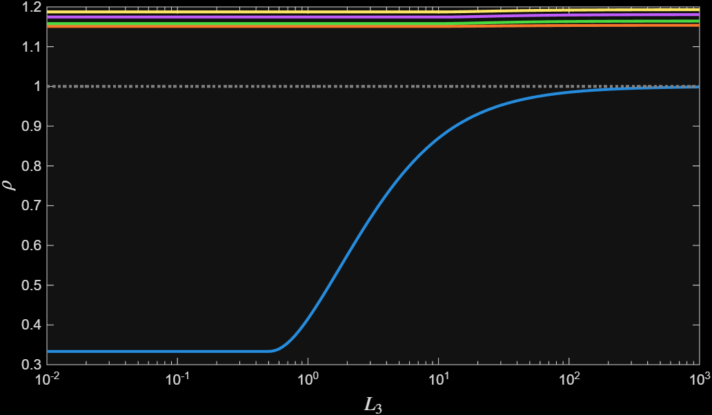
Figure 1: Davis-Yin with \(\gamma = 1/{L_3}\) with delays#
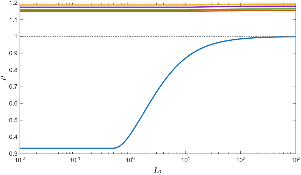
Figure 1: Davis-Yin with \(\gamma = 1/{L_3}\) with delays#
Figure 2 plots the same curves with Davis-Yin parameters \(\gamma = 1/(2{L_3}), \lambda = 0.\)
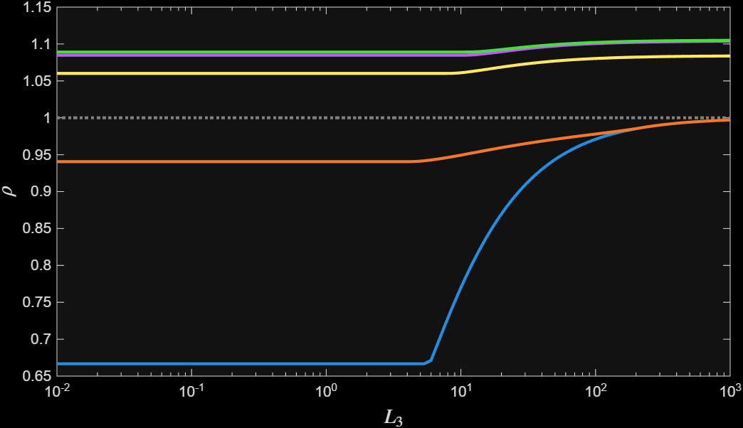
Figure 2: Davis-Yin with \(\gamma = 1/(2{L_3})\) with delays#
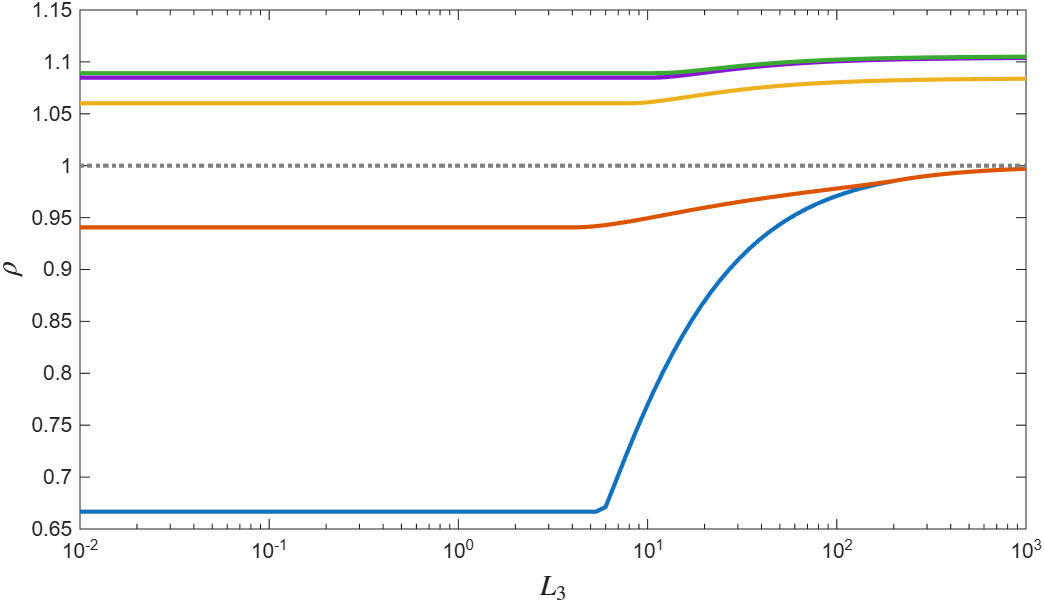
Figure 2: Davis-Yin with \(\gamma = 1/(2{L_3})\) with delays#
 1%sweep of L3
 2NL = 100;
 3L_all = logspace(-2, 3, NL);
 4
 5%define base operators
 6m = [0, 1, 0];
 7L = [inf, 1.5, inf];
 8ops= cell(1, 3);
 9for i = 1:3
10    ops{i} = op_sml(m(i), L(i));
11end
12
13%outer loops
14orderlist = {0, 1, [0, 1], [1, 1], 2, [0, 2]};
15delaylist = 0:4;
16Ndelay = length(delaylist);
17Norder = length(orderlist);
18
19rho_best = zeros(NL, 1);
20rho_bound = zeros(NL, Norder, Ndelay);
21parfor j = 1:NL
22    for k = 1:Ndelay
23        delay = delaylist(k);
24        ops_curr = ops;
25        ops_curr{3}.L = L_all(j);
26
27        %davis-yin algorithm
28        lambda = 1;
29        gamma = 1/L(2); % or gamma = 1/(2*L(2));
30        K = ss([1], [-gamma*lambda, -gamma*lambda, -gamma*lambda], [1; 1; 1], ...
31            [-gamma, 0, 0; ...
32            -gamma, 0, 0; ...
33            -2*gamma, -gamma, -gamma],1);
34
35        %form the system
36        network = bridge_channel_delay([0, delay, 0], [0, delay, 0]);
37        sys = opt_system(ops_curr, network, K);
38
39        %perform analysis at each order
40        man = opt_analysis(sys);
41        for i = 1:Norder
42            order_curr = repmat({orderlist{i}}, 1, 3);
43            sol = man.bisect(order_curr);
44            rho_bound(j, i, k) = sol.rho;
45        end
46    end
47end
48
49
50%% plot the result
51
52
53figure(1)
54clf
55plot(L_all, squeeze(rho_bound(:, 4, :)), 'linewidth', 2);
56hold on
57    set(gca, 'Xscale', 'Log')
58    ylabel('$\rho$', 'interpreter', 'latex','Fontsize', 14)
59    xlabel('$L_3$', 'interpreter', 'latex','Fontsize', 14)
60    xlim([L_all(1), L_all(end)])
61
62plot(L_all, ones(size(L_all)), ':', 'LineWidth', 2, 'color', 0.5*[1,1,1])