Coordinate Descent

This examples Synthesizes cyclic coordinate descent algorithms, continuing from the previous simulation and Analysis examples.

Two types of cyclic coordinate descent algorithms are the considered in this demonstration:

1. Full Knowledge: the entire vector \(\nabla f(\beta_k)\) is known,

2. Partial Knowledge: only the actively updated portion \([\nabla f(\beta_k)]^i\).

The reference coordinate descent algorithm in the prior examples is

\[\begin{align} \beta^{i(k)}_{k+1} = \beta^{i(k)}_{k} -\gamma \ [\nabla f(\beta_k)]^i. \end{align}\]

This reference algorithm has Partial Knowledge.

Synthesis is performed to design a \(c\)-block cyclic coordinate descent algorithm with respect to a function \(f \in S_{1, 2}\). Figure 1 plots the upper bounds on the convergence rate \(\rho\) as \(c\) increases. Algorithms with Partial Knowledge (orange, top) have a higher worst-case convergence rate when compared against algorithms with Full Knowledge (blue, bottom) at \(c>1\). The two synthesized algorithms are equal in the trivial case of \(c=1\).

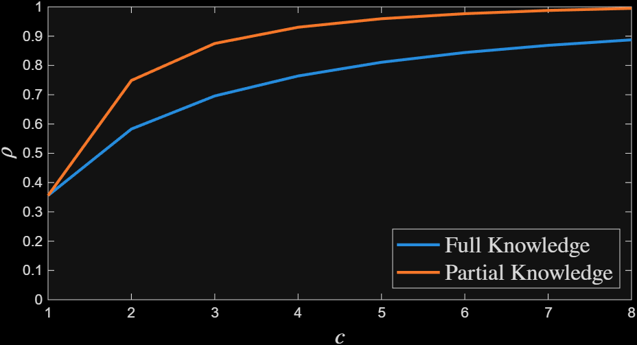
Figure 1: Convergence rate of coordinate descent algorithm v.s. number of blocks

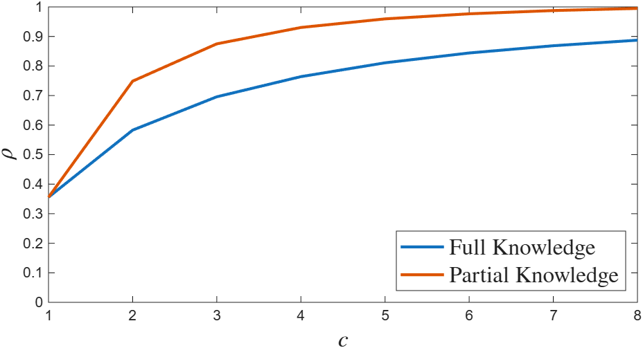
Figure 1: Convergence rate of coordinate descent algorithm v.s. number of blocks.

Code for coordinate descent synthesis at \(m=1, L=2, c=6\)

c=6; %blocksize 

%symmetry generator/permutation matrix
M = circshift(eye(c), 1); 

%define the objective function
m = 1; L = 2; 

op1 = op_sml(m, L);

op1.c = c; %enforce coordinate dimension

%performs gradient operations, not prox
config = opt_config();
config.syn.D_mask = 0;

%% Full Knowledge
network = coordinate_descent_system(c);

%form the system
sys = opt_system_periodic_orbit(op1, network, [], M);

man = opt_synthesis(sys, config);

% %access to all parts of gradient
sol = man.bisect();