Stochastic Gradient Noise

This example performs Analysis of the Projected Gradient Descent (PGD) algorithm to solve the composite optimization problem \(\min f(\beta) + g(\beta)\). The gradients of the function \(f \in S_{m, L}\) are corrupted by additive stochastic noise. The p.c.c. function \(g\) is unaffected by noise. The additive noise \(w_{p, k}\) is i.i.d. normally distributed at each time, with matrix covariance \(\Omega\). The performance output is the error \(z_{p, k} := z^2_k - \beta^*\). The resulting

The representation of the noise-corrupted PGD algorithm used for Stochastic analysis is

\[\begin{split}\begin{align*} \mat{c}{x_{k+1} \hl z_k^1 \\ z_k^2 \\ z_{p, k}} &= \mat{c|cc:c}{I & - \gamma I & -\gamma I & -\gamma I \hl I &- \gamma I & 0 & 0 \\ I &- \gamma I & 0 & 0 \hdl I &- \gamma I & 0 & 0 } \mat{c}{x_{k} \hl w_k^1 \\ w_k^2 \hdl w_{p, k}}, & \mat{c}{w_k^1 \\ w_k^2} \in \mat{c}{\partial g_(z_k^1) \\ \nabla f(z_k^2)}. \end{align*}\end{split}\]

This representation ensures that the performance input \(w\) never enters an oracle evaluation \(\partial g\) or \(\nabla f\).

Analysis is performed with paramters \(m = 1, L = 10, \Omega = I\). The stepsize parameter \(\gamma\) is swept in the range \([0, \frac{2}{L+m}\). The Stochastic Sensitivity and convergence rate are computed for each \(\gamma\) using an Analysis program with orders [1, 1] at each oracle. Figure 1 plots the results of two executions of Analysis. The Separate Search poses and solves two separate Analysis. The Joint Search solves a single multi-criteria Analysis program. The conservatism of the joint approach is illustrated by the difference between the curves.

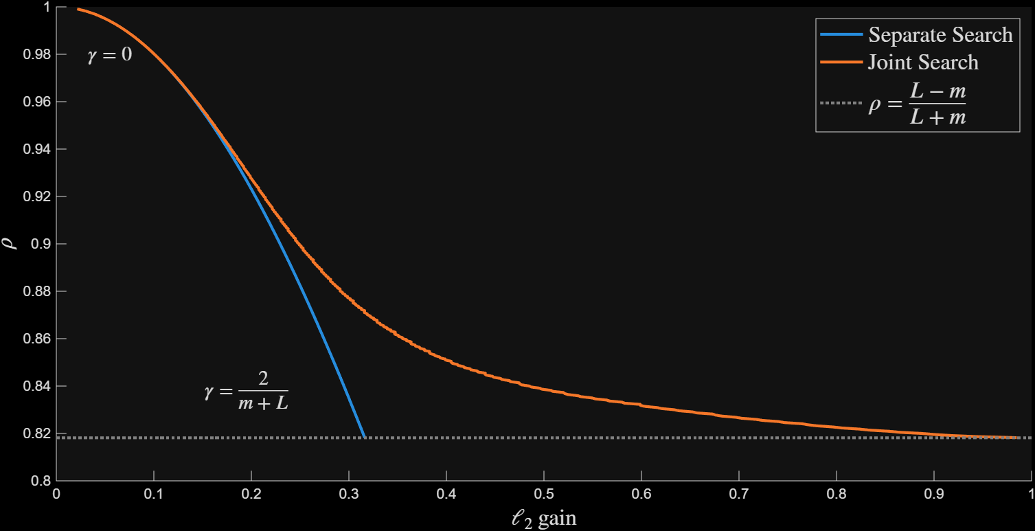
Figure 1 Convergence rate v.s. sensitivity

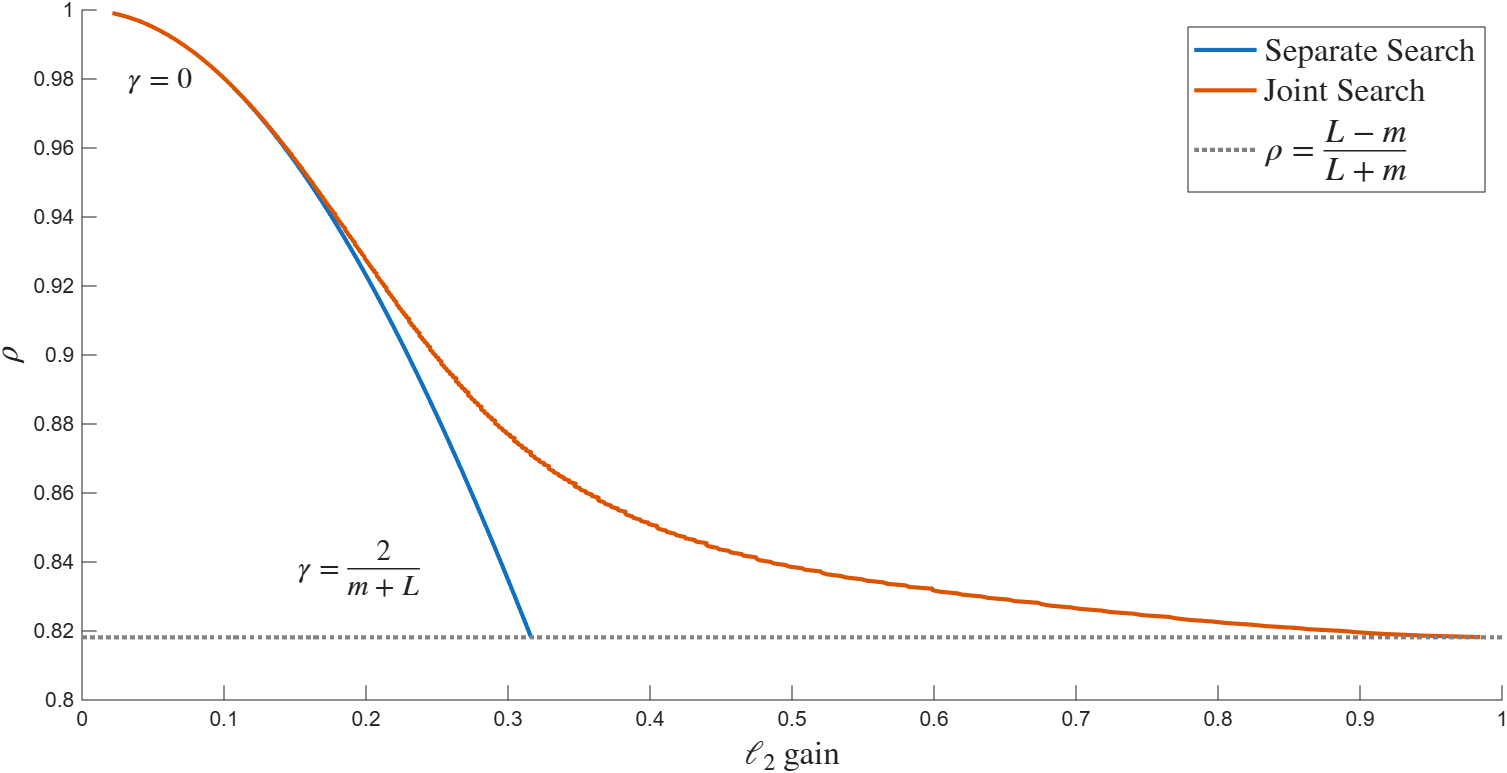
Figure 1: Convergence rate v.s. sensitivity

Code for Analysis with stochastic gradient noise

%define the operators
m = 1;L = 10;
op1= op_pcc(); %pcc goes first, to not take information from the noisy gradient
op2= op_sml(m, L);
ops = {op1, op2};

%define the PGD
gamma = 2/(L + m);
K = ss(1, [-gamma, -gamma], [1; 1], [-gamma, 0; -gamma, 0],1);

%gain from (error in w2) to (z2 - z*)
network = bridge_pass_through(2); %start with no network dynamics
[network, iwp] = network.add_oracle_input(2, []); %add wp
[network, izp] = network.perf_output_z(2); %add zp

%define specification
GAIN = 10;
spec_stoch = spec_h2(GAIN, 1, iwp, izp);
spec_stoch.target = true;


%form the systems
sys_clean = opt_system(ops, [], K); %for convergence rate
sys_noisy = opt_system(ops, network, K); %for stochastic sensitivity

%pose the analysis problem
order = {1, 1};

%only convergence
man_noisy= opt_analysis(sys_noisy);
sol_noisy = man_noisy.solve_single(order, spec_stoch);

%only sensitivity
man_clean = opt_analysis(sys_clean);
sol_clean = man_clean.bisect(order);

%both at once: minimize rho with inner objective h2 gain
specs_joint = {spec_stability(1), spec_stoch};
man_joint = opt_analysis(sys_noisy);
sol_joint = man_joint.bisect(order, specs_joint);


h2gain = sqrt(sol_noisy.objective); %  0.3162
rho = sol_clean.rho; % 0.8182

h2gain_joint = sqrt(sol_joint.objective); % 1.0389
rho_joint = sol_joint.rho; % 0.8182