Noisy Unstable Network

This example solves a composite optimization problem with three functions

\[\beta^* \in \argmin f(\beta) + \frac{1}{2}\norm{\beta - b_0}_2^2 + \mathbb{I}_{\mathcal{Z}}(\beta)\]

The three functions in the sum are respectively in the classes \(S_{m, L}, S_{1, 1}, S_{0, \infty}\).

The evaluation of \(\nabla f\) is inexact \((w = \nabla f(z) + w_p)\), and the transmission of these noisy gradients occur over an unstable communication channel

\[\begin{split}\begin{align*} \mat{c}{x^N_{k+1} \hl z^1_k \\ y^1_k} = \mat{cc|cc}{1.2 I & 0 & I & 0\\0 & -0.2 I & 0 & I \hl 0 & I & 0 & 0 \\ I & 0 & 0 & 2 I} \mat{c}{x^N_{k} \hl w^1_k \\ u^1_k}. \end{align*}\end{split}\]

Synthesis is performed with \(m=1, L=3\). Only the nonsmooth term \(\mathbb{I}_{\mathcal{Z}}\) is evaluated implicitly. The overall algorithm satisfy an \(\ell_2\)-stability specification at minimal rate \(\rho\).

The resulting controller has a worst-case performance of \(\rho < 0.9896\). The algorithm is simulated starting at \(x_0=0\), for a problem where \(f\) is a randomly generated quadratic and \(\mathcal{Z}\) is an \(L_1\)-ball with radius \(50\).

Figure 1 plots the function values, and errors over the execution with \(w_p = 0\).

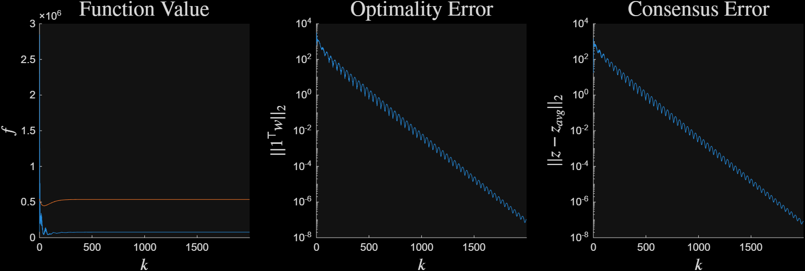
Figure 1: Trace of function values and errors

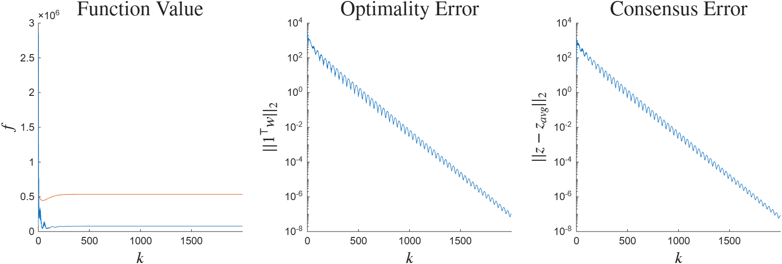
Figure 1: Trace of function values and errors

Figure 2 plots the states, oracle input, oracle output over this execution.

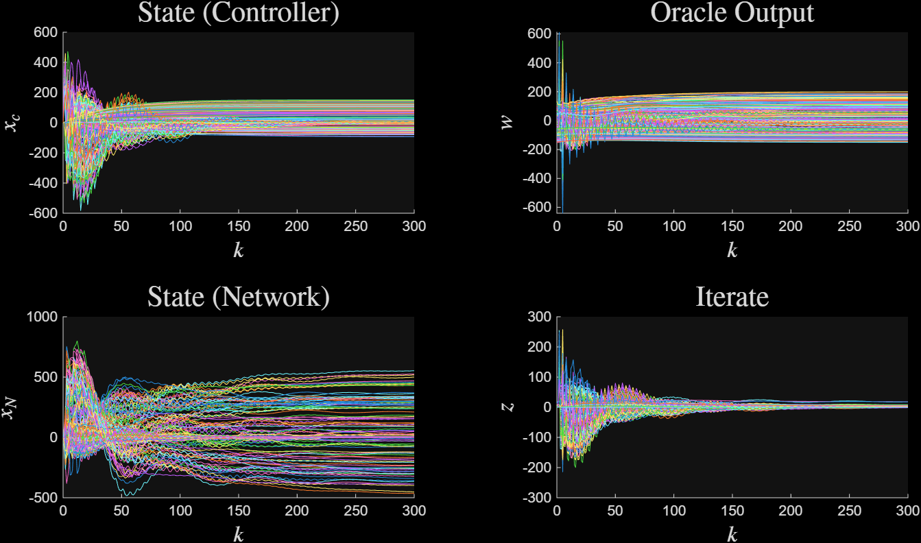
Figure 2: Trace of state and oracle evolution

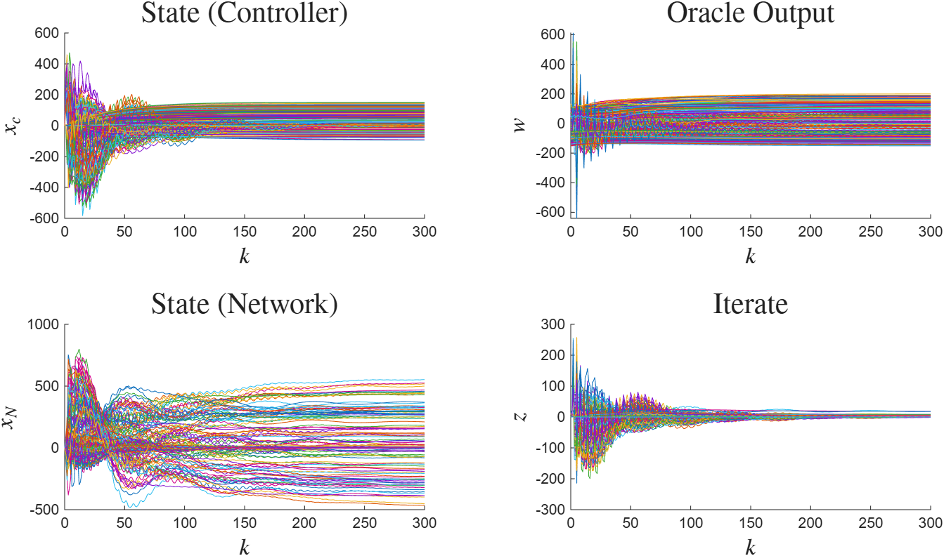
Figure 2: Trace of state and oracle evolution (noiseless)

Figure 3 plots the tracking errors of the algorithm based on the Regulator Equation solutions.

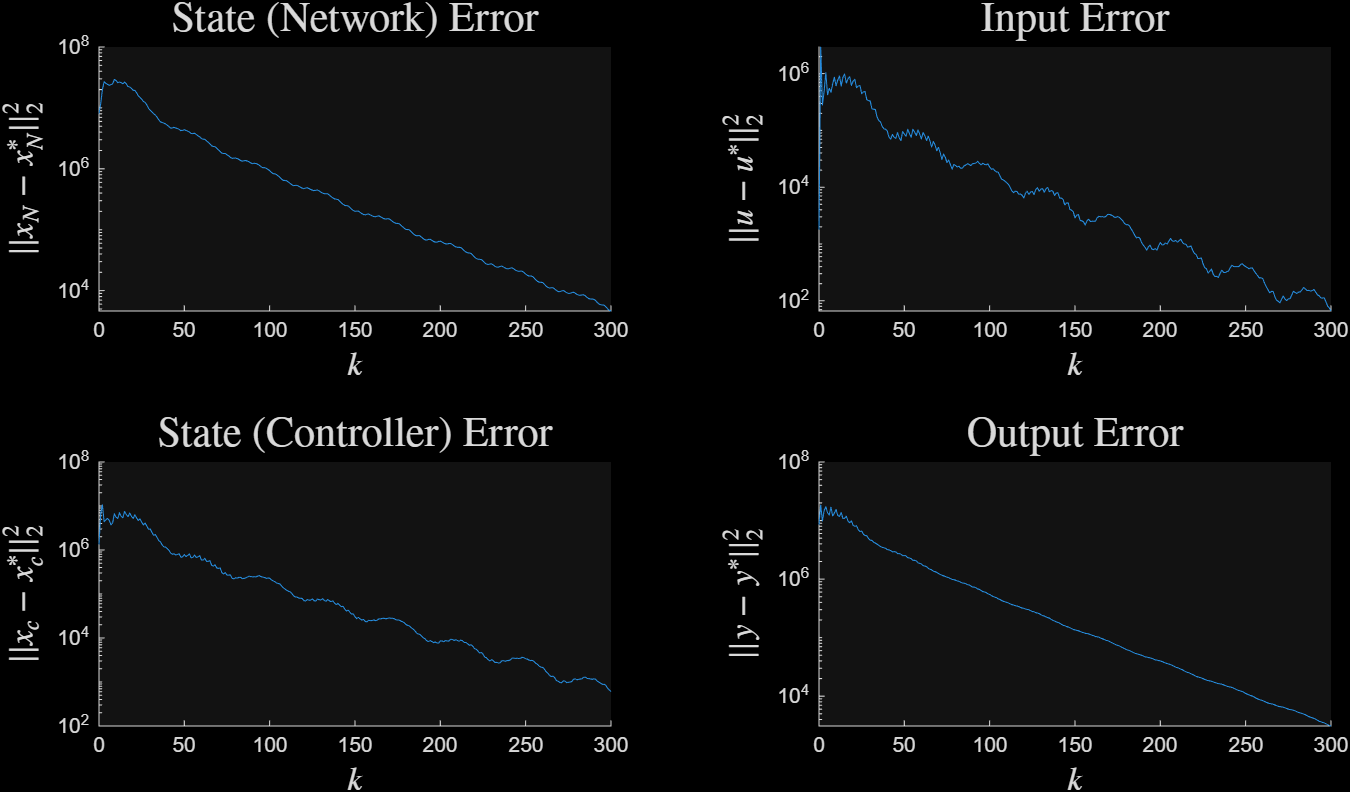
Figure 3: Trace of tracking errors (noiseless)

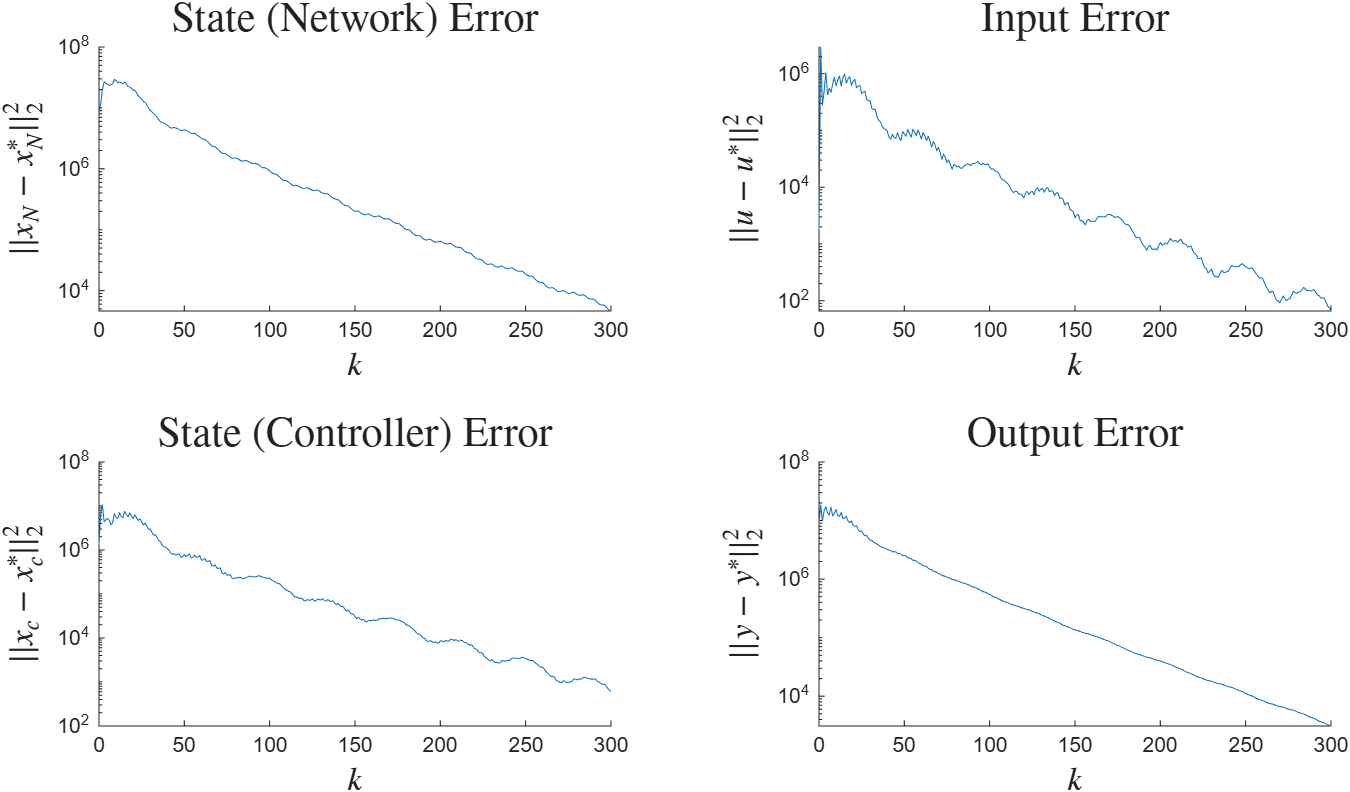
Figure 3: Trace of tracking errors (noiseless)

Noise is now injected into the gradient evaluation. The applied performance input \(w_p\) is bounded as \(\max_{k \in \{0, \ldots, T\}} \norm{w_{p, k}}_2^2 \leq 10\) for all time horizons \(T \in \N\). Figure 4 plots the persistent tracking and convergence errors with this exogenous noise.

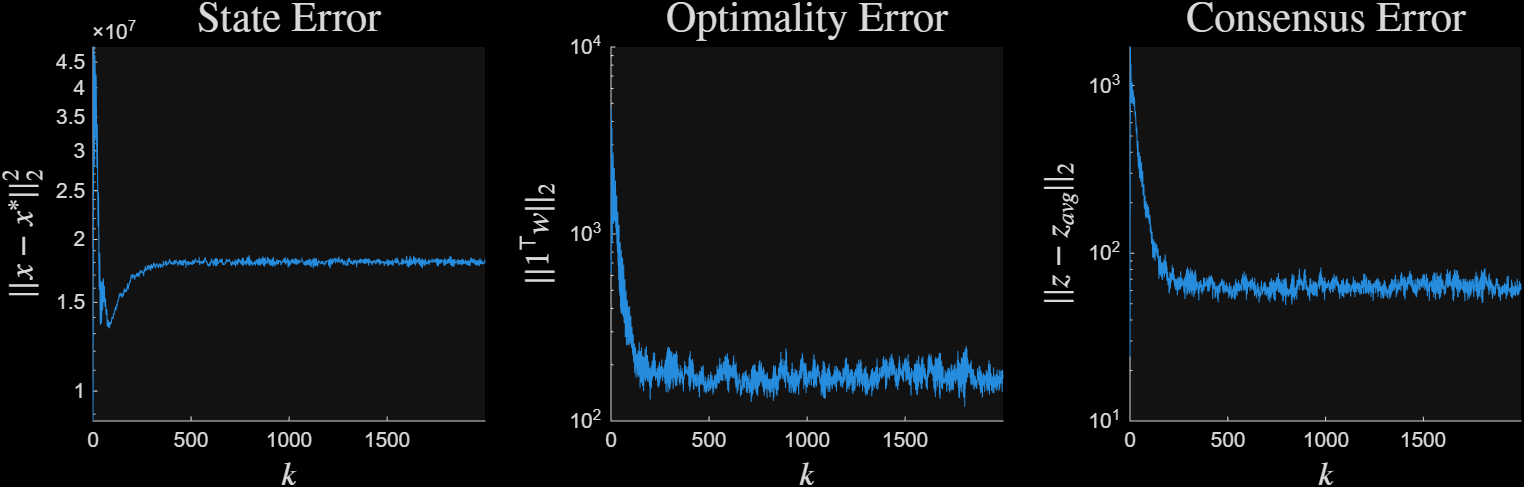
Figure 4: Trace of tracking, optimality, and consensus errors (noisy)

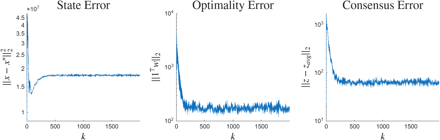
Figure 4: Trace of tracking, optimality, and consensus errors (noisy)