Channel Memory

This example involves a two-operator inclusion problem. Memory effects are present in the communication link to and from evaluation of \(F_1\). The intensity of the memory effects are represented by a scalar forgetting factor \(\alpha > 0\). The network effects for all \(k \in \N\) are

\[\begin{split}\begin{align*} z^1_k &= u_k^1 - \alpha z^1_{k-1}, & y_k^1 &= w_k^1 - \alpha y_{k-1}^1, \\ z^2_k &= u_k^2, & y_k^2 &= w_k^2. \end{align*}\end{split}\]

The degenerate case of \(\alpha=0\) is no network dynamics. A state-space realization of these memory effects is

\[\begin{split} \text{Network}: \qquad \mat{c}{x_{k+1}^N \hl z_k \hdl y_k} = \mat{cc|cc:cc}{-\alpha I & 0 & \frac{1}{2} I & 0 & 0 & 0 \\ 0 & -\alpha I & 0 & 0 & \frac{1}{2}I & 0 \hl 0 & -2\alpha I & 0 & 0 & I & 0 \\ 0 & 0 & 0 & 0 & 0 & I \hdl -2 \alpha I & 0 & I & 0 & 0 & 0 \\ 0 & 0 & 0 & I & 0 & 0} \mat{c}{x_{k}^N \hl w_k \hdl u_k}.\end{split}\]

The controller structure with parameters \((\gamma, \lambda) \geq 0\) used to solve the two-operator inclusion problem is

\[\begin{split} \mat{c}{x_{k+1}^c \hl u_k^1 \\ u_k^2} = \mat{c|cc}{I & -\gamma \lambda & \frac{ -\gamma \lambda}{\alpha+1} \hl (1+\alpha) I & 0 & 0 \\ I & -\gamma I & -\frac{ -\gamma }{\alpha+1} I } \mat{c}{x_{k}^c \hl y_k^1 \\ y_k^2}.\end{split}\]

This controller structure is parameterized by \(\alpha\). If \(\alpha = 0\) and \(\lambda = 1\), then this controller is the same as Projected Gradient Descent. The controller structure is chosen to ensure that the Regulator Equation condition for algorithm convergence is satisfied for all values \((\gamma, \lambda)\). Projected Gradient Descent fails the regulator equation requirement of convergence when \(\alpha > 0\).

We use this algorithm to solve a composite optimization problem

\[\beta^* \in \argmin_{\norm{\beta}_1 \leq 100 } f(\beta)\]

where \(f\) is a convex quadratic with \(m=1\), \(L=5\).

Figure 1 plots a trace of algorithm execution starting from \(x_0 = 0\), highlighting the states of the network and controller.

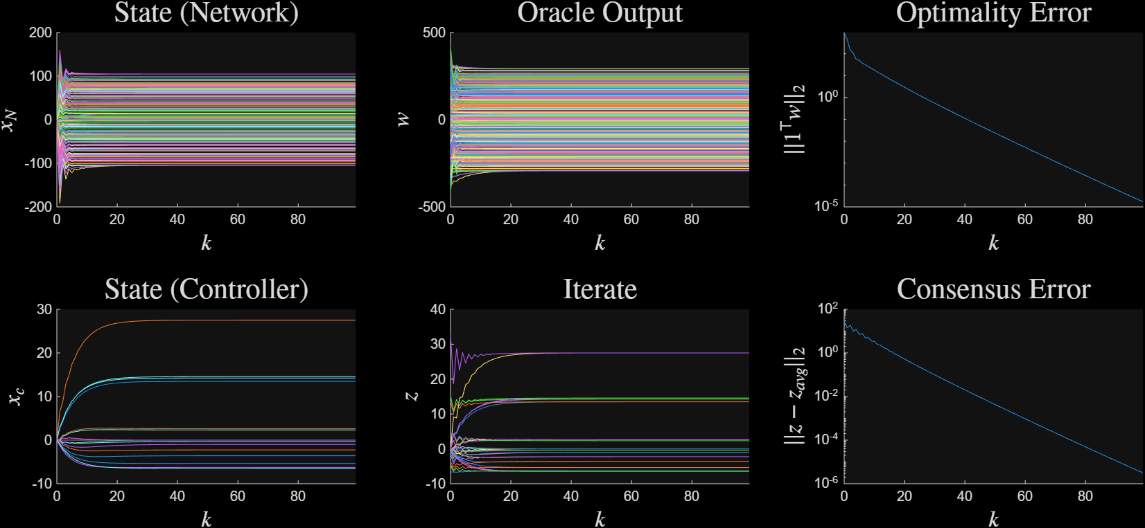
Figure 1: Trace of execution and convergence

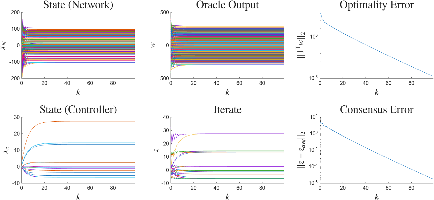
Figure 1: Trace of execution and convergence

The Regulator Equations are used to establish tracking properties of solution trajectories. The solution to the Regulator Equations for this network and controller are

\[\begin{split}\begin{align*} \Pi &= \mat{cc}{0 & \frac{1}{2(\alpha+1)}I \\ -\frac{1}{2} I & 0 }, & \Gamma &= \mat{cc}{-(\alpha+1) I & 0 \\ -I & 0 }, \\ \Phi &= \mat{cc}{0 & \frac{1}{2(\alpha+1)}I \\ 0 & -I }, & \Theta &= \mat{c}{-I & 0}. \end{align*}\end{split}\]

The pair \((\beta^*, w^*)\) solving the composite optimization problem is unique, because \(f\) is strongly convex with a nonempty constraint set is nonempty, and \(f\) is smooth. Algorithm convergence implies tracking of the signals \((x^N, x^c, y, u)\) with

\[\begin{split}\begin{align*} \lim_{k \rightarrow \infty} \mat{c}{x_k^N \\ x^c_k \hl y_k \\u_k} & = \mat{c}{\Pi \\ \Theta \hl \Phi \\ \Gamma} \mat{c}{-\beta^* \\ \nabla f(\beta^*)}. \end{align*}\end{split}\]

Figure 2 plots the tracking of these signals over time

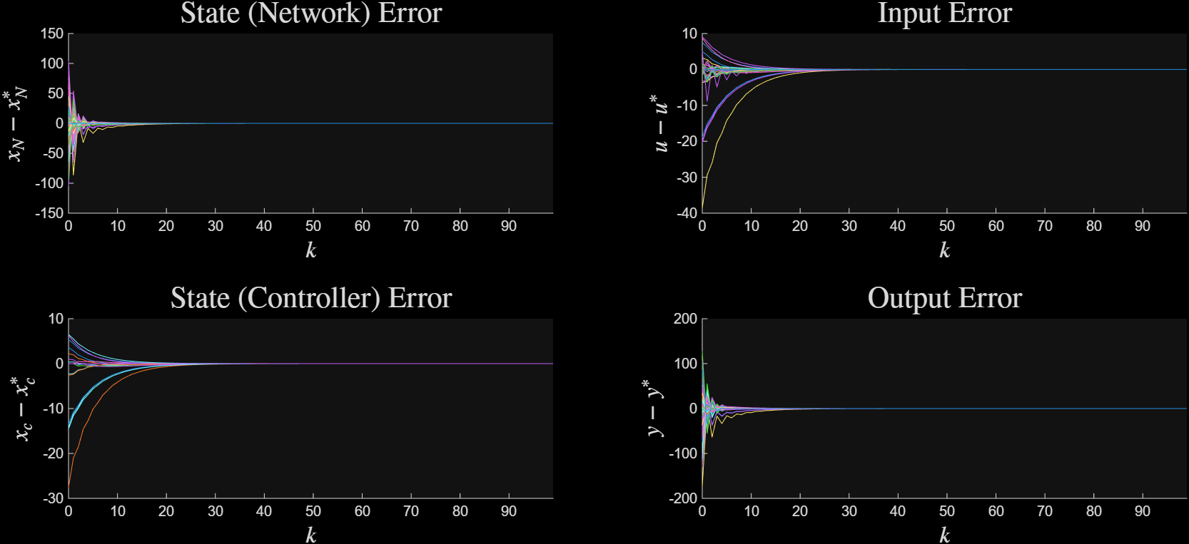
Figure 2: Tracking errors

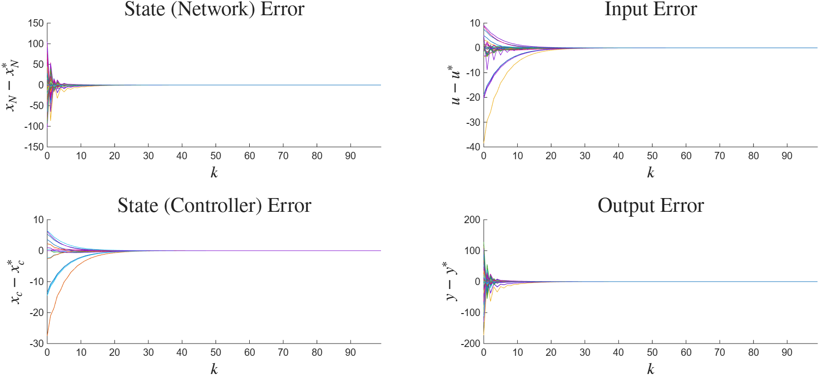
Figure 2: Tracking errors

Figure 3 plots the squared norm of the tracking error

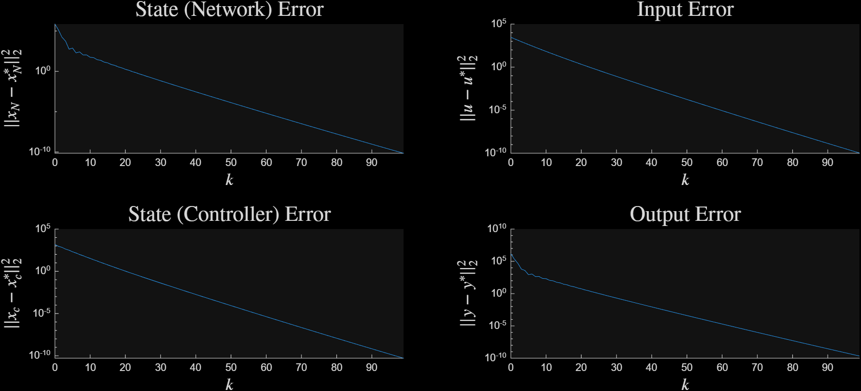
Figure 3: Tracking residuals

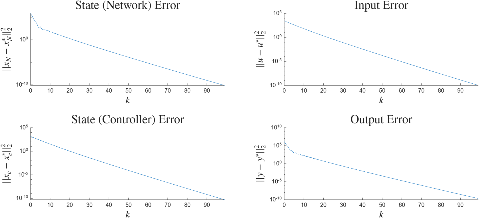
Figure 3: Tracking residuals

See also

Analysis of the channel-memory algorithm.