

Cyclic Coordinate Descent#
A coordinate descent algorithm searches over only a subset of variables in each iteration. [1].
Letting \(i(k)\) be the active coordinate block at iteration \(k\), a coordinate descent method to minimize a function \(f\) is with stepsize \(\gamma>0\) is
This coordinate descent algorithm is used to solve an unconstrained optimization problem \(\min_{\beta \in \R^{90}} f(\beta)\). The function \(f\) is parameterized by scalars \(0 < m < W < L\), a constant vector \(b\), and a symmetric matrix \(Q\) with eigenvalues between \(m\) and \(W\). The non-quadratic function \(f \in S_{m, L}\) is
Coordinate descent with \(\gamma = 0.1\) is performed starting from an initial condition \(x_0 = 0\). The \(c=6\) coordinate blocks are updated cyclically in increasing order.
Figure 1 plots a short trajectory of cyclic coordinate descent.
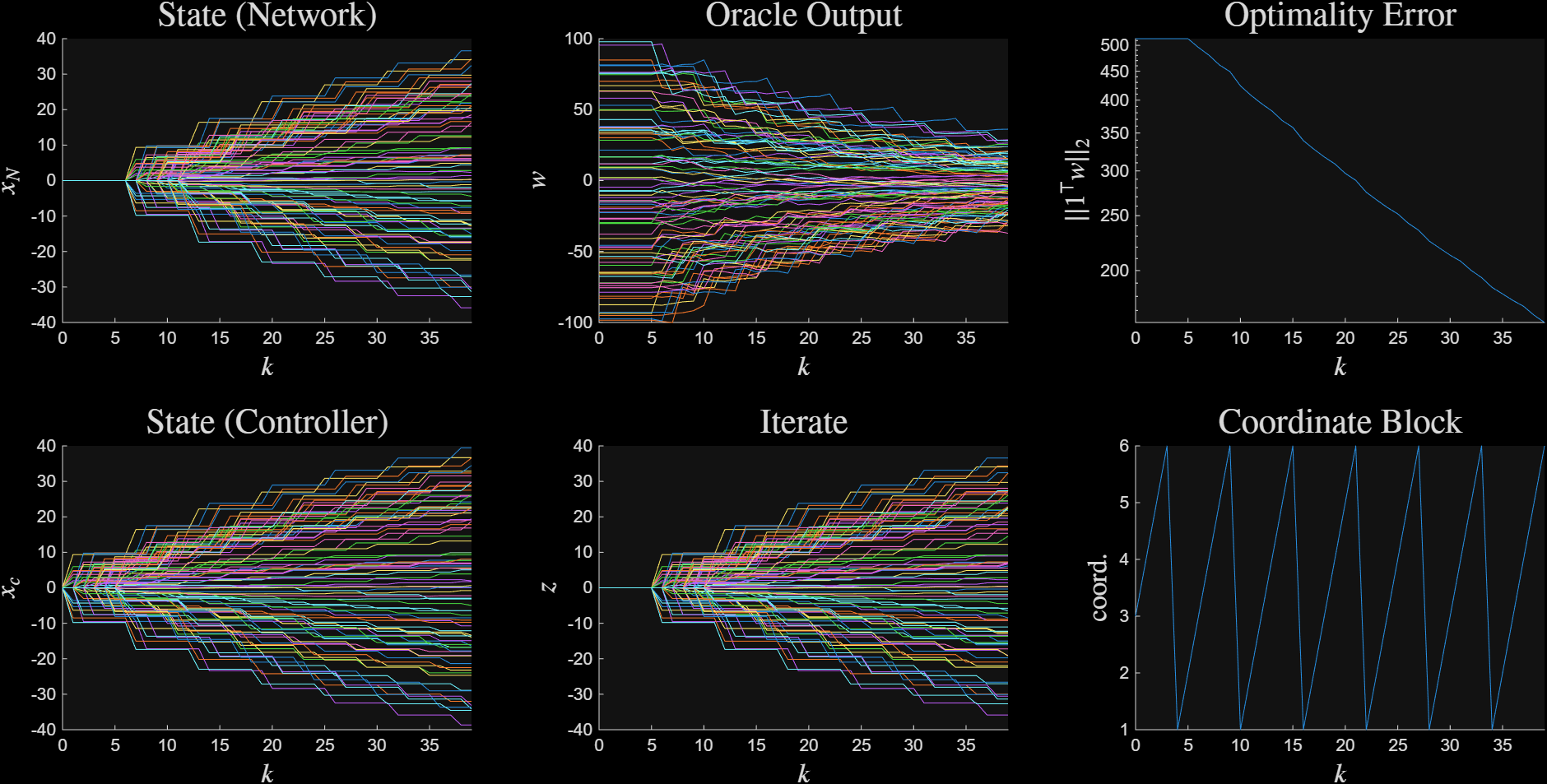
Figure 1: Convergence of coordinate descent algorithm (short time horizon)#
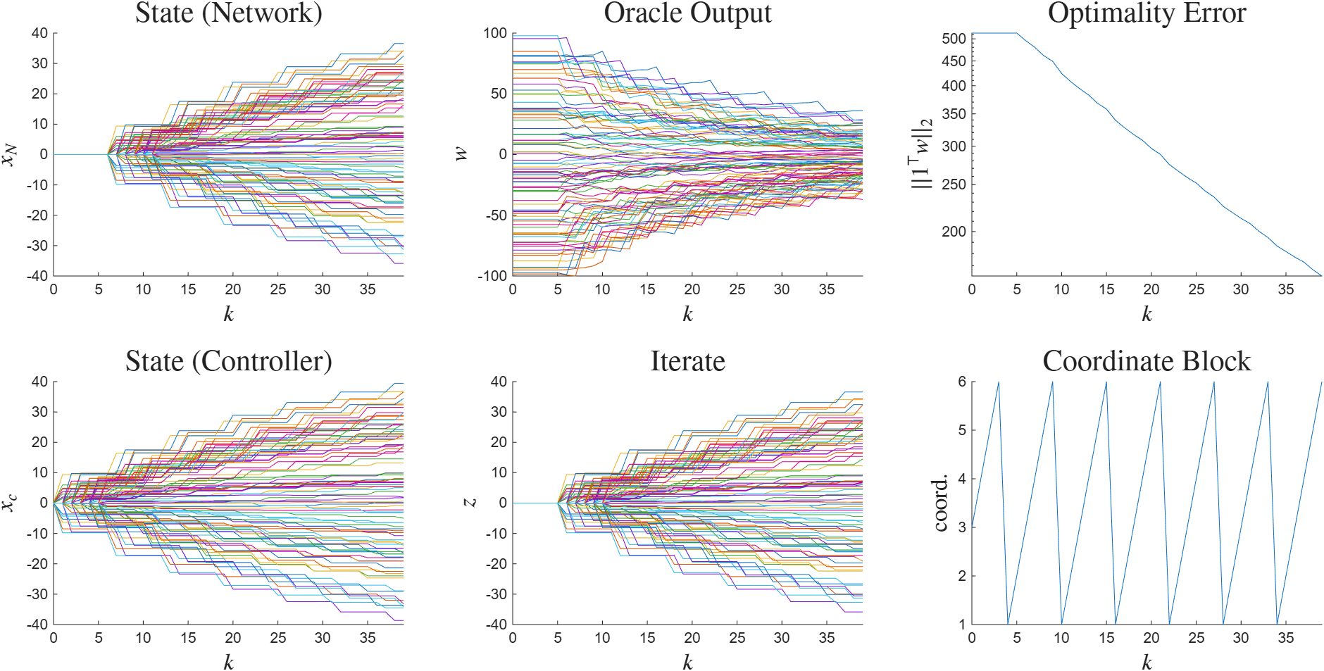
Figure 1: Convergence of coordinate descent algorithm (short time horizon)#
Periodic-Orbit Construction#
Cyclic coordinate descent schemes can be modeled as Periodic-Orbit Systems. Given a block-size \(c\), we define the permutation matrix
The \(c\)-block cyclic coordinate descent algorithm with \(\gamma>0\) is described by
Algorithm simulation is performed by using the opt_system_periodic_orbit object.
 1%coordinate descent scheme
 2rng(50, 'twister');
 3
 4d = 30; %number of dimensions
 5c = 5;
 6
 7%symmetry generator/permutation matrix
 8M = circshift(eye(c), 1);
 9
10%gradient descent rule
11gamma = 0.2;
12
13K = ss(eye(c), -gamma*eye(c), ...
14    eye(c), zeros(c), 1);
15
16%define the objective function
17%sum of quadratic and log-sum-exp
18m = 1; L = 5; L2 = 3;
19Q = rand_quad(d, m, L2);
20bstar = 100*(2*rand(d, 1) - 1);
21
22fw_func = @(k, z, param) Q*z + bstar + (L - L2)* (exp(z) - exp(-z)) / sum(exp(z) + exp(-z));
23bw_func = @(k, z, D, param) []; %unused
24f_func =  @(k, z, param) 0.5*z'*Q*z + bstar' * z + (L - L2)*log(sum(exp(z) + exp(-z)));
25op1 = op_sim(fw_func, bw_func, f_func);
26
27op1.c = c; %enforce coordinate dimension
28
29%define the network
30%implements coordinate descent
31n = struct('nu', c, 'ny', c, 'nz', c, 'nw', c);
32network = genplant([zeros(c), eye(c); blkdiag(1, zeros(c-1)), zeros(c)], n);
33
34%form the system
35sys = opt_system_periodic_orbit(op1, network, K, M);
36% sys = opt_system_periodic_orbit(op1, [], alg, M);
37reg = regulator_periodic_orbit(sys);
38rcl = reg.check_regulator();
39
40%% simulate coordinate descent
41sim = alg_sim(sys, d);
42T = 51;
43sim_out= sim.sim(T);
44
45% T_long = 801;
46% sim_out_long= sim.sim(T_long);
47
48
49%% plot
50plt = alg_plotter(sim_out);
51plt.plot({'f', 'w', 'res_w', ...
52    'x', 'z', 'coord', }, 10);
53
54% plt_long = alg_plotter(sim_out_long);
55% plt_long.plot({'xn', 'w', 'res_w', ...
56%     'xc', 'z', 'coord', }, 2);