Coordinate Descent Algorithms

This example continues the coordinate-descent simulation demonstration.

A function \(f \in S_{m, L}\) is optimized using a \(c\)-block cyclic coordinate descent algorithm with gradient steps.

Analysis is performed for this gradient descent scheme

\[\begin{align} \beta^{i(k)}_{k+1} = \beta^{i(k)}_{k} - \gamma \ [\nabla f(\beta_k)]^i \end{align}\]

with stepsize \(\gamma := \frac{2}{c(m+L)}\). The coordinate block size \(c\) is increased from 1 to 6, and the parameter \(L\) is swept from 1 to 100 while \(m\) is kept to 1. Figure 1 plots the \(\rho\) upper bounds computed at order [1, 0].

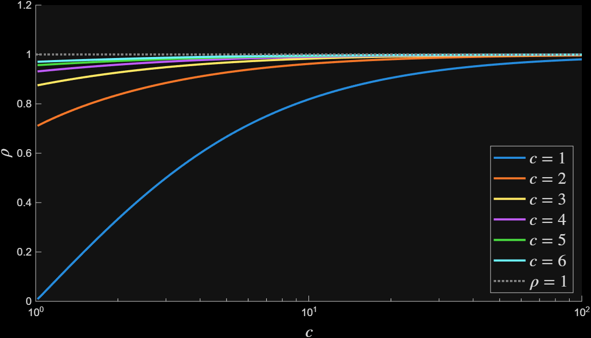
Figure 1: Convergence rate of coordinate descent algorithm v.s. number of blocks

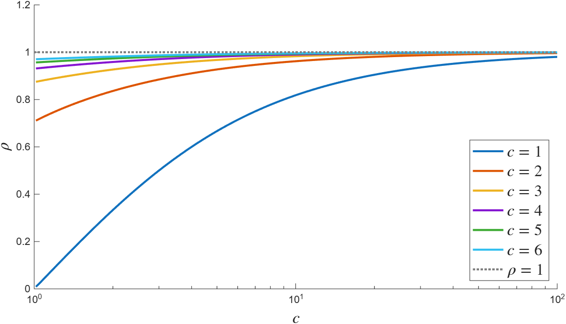
Figure 1: Convergence rate of coordinate descent algorithm v.s. number of blocks.

The specific analysis code at \(m=1, L=5, c=4\) is

Code for coordinate descent analysis

c=4; %blocksize

%symmetry generator/permutation matrix
M = circshift(eye(c), 1); 

%operator definition
m = 1; L = 5;
op1 = op_sml(m, L);

%gradient descent rule
%coordinate updates
gamma = 2/(L +m) * (1/c); 
K = ss(eye(c), blkdiag(-gamma , zeros(c-1)), ...
    eye(c), zeros(c), 1);

%form the system
sys = opt_system_periodic_orbit(op1, [], K, M);

% %simulate and plot
man = opt_analysis(sys);

order = [2, 1]; 
sol = man.bisect(order); %0.8942