Time-Varying Delay

This example simulates a Projected Gradient Descent algorithm subject to time-varying delays. We aim to solve the constrained optimization problem

\[\beta^* \in \argmin_{\norm{\beta}_\infty \leq 10} f(\beta),\]

where \(f\) is a convex quadratic with eigenvalues between \(m=1\) and \(L=1.5\).

A time-varying delay \(h(k)\) is introduced after evaluation of \(\nabla f\). The expression for PGD with time-delays is

\[\begin{split}\begin{align*} \mat{c}{x_{k+1} \hl z_k^1 \\ z_k^2} &= \mat{c|cc}{I & -\gamma I & -\gamma I \hl I &0 & 0 \\ I & -\gamma I & -\gamma I } \mat{c}{x_{k} \hl w_{k-h(k)}^1 \\ w_k^2}, & \mat{c}{w_{k}^1 \\ w_k^2} \in \mat{c}{\nabla f(z_k^1) \\ \partial I_{\norm{\cdot}_\infty \leq 10}(z_k^2)} \end{align*}.\end{split}\]

The delay \(h(k)\) is bounded between 0 and 3 steps at all \(k \in \N\). It is temporally restricted according to the logics

Type	Rule
Periodic	\(h(k)\) increases by 1, and drops to 0 if \(h(k)=0\).
Snap	\(h(k)\) either increases by 1 or drops to 0, but \(h(k+1)=0\) always holds if \(h(k)=3\).
Contiguous	\(h(k)\) increases by 1, stays the same, or decreases by 1, subject to the constraint \(h(k) \in [0, 3]\).

The Snap logic is motivated by communication failures: PGD will use the same stale gradient until a successful transmission is received. Snap and Contiguous are nondeterministic switching logics, while Periodic is deterministic given \(h(0)\).

We solve the composite optimization problem using a nominal PGD algorithm with stepsize \(\gamma = 0.05\). All executions are performed starting at \(x_0=0\), and at a random initial delay \(h(0)\). Figure 1 plots the algorithm trajectory under periodic time-varying delays.

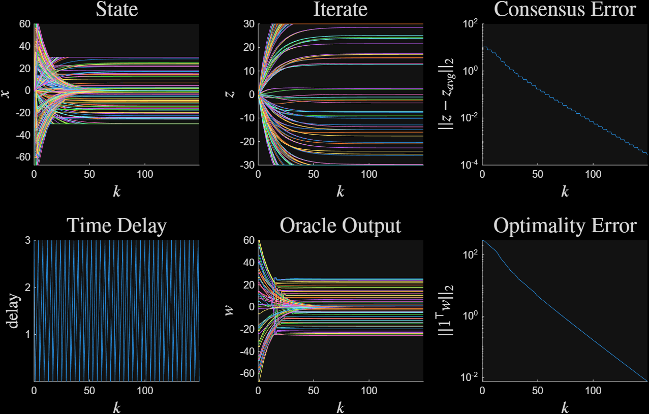
Figure 1 Periodic time delays

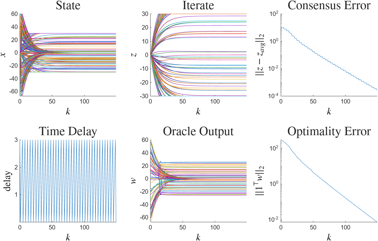
Figure 1: Periodic time delays

Figure 1 plots the algorithm trajectory under periodic time-varying delays.

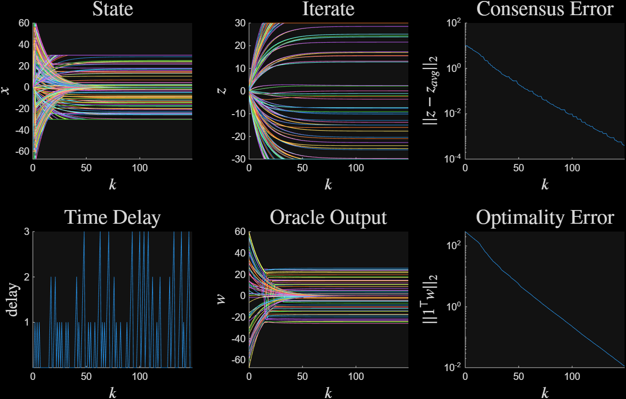
Figure 2 Snap time delays

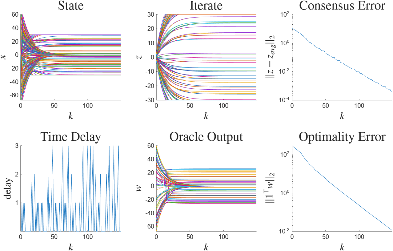
Figure 2: Snap time delays

Figure 3 plots the algorithm trajectory under contiguous time-varying delays.

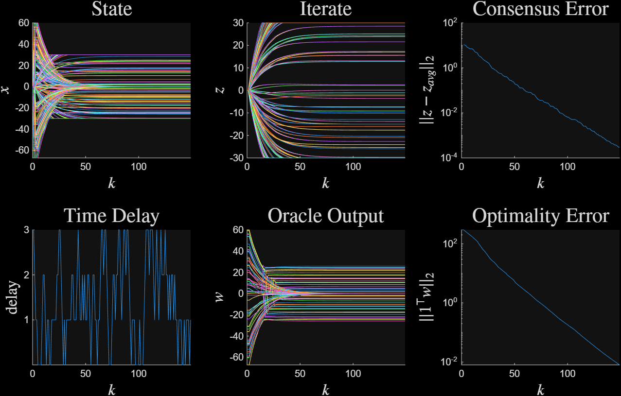
Figure 3 Contiguous time delays

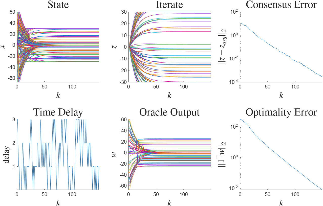
Figure 2: Contiguous time delays

Code for Projected Gradient Descent with time-varying delays

%time-varying delays
rng(40, 'twister');
d = 64;
delay_max = 3;


%% define the operators
%generate the test quadratic
m = 1; L = 1.5;
Q = rand_quad(d, m, L);
bstar = randi(101, [d, 1]) - 50;
op1 = op_sim_quad(Q, bstar);

%indicator function 
BOX = 30;
op2 = op_sim_box(BOX);

ops = {op1, op2};

%% form the time-varying delay network

%delay for oracle 1
[Pprim, Gcon] = delay_primitives(0, 0:delay_max, 0,  -1:1);
Gsnap = delay_snap_graph(delay_max, 0);

%no delay for oracle 2
P0 = bridge_pass_through(1);

%build the network by block diagonalization
Nss = length(Gsnap);
P_chain = cell(Nss, 1);
for i = 1:Nss    
    P_chain{i} = blkdiag(Pprim{i}, P0);
end

network = genplant_poly(P_chain);

%projected gradient descent
gamma = 0.05;
K = ss([1], [-gamma, -gamma], [1; 1], [0, 0; -gamma, -gamma],1);

%form the systems
sys_per = opt_system_periodic(ops, network, K);
sys_snap = opt_system_switched(ops, network, K, Gsnap);
sys_cont = opt_system_switched(ops, network, K, Gcon);


%% begin simulation
T = 150;
sim_per  = alg_sim(sys_per, d);
sim_snap = alg_sim(sys_snap, d);
sim_cont = alg_sim(sys_cont, d);


sim_out_per  = sim_per.sim(T);
sim_out_snap = sim_snap.sim(T);
sim_out_cont = sim_cont.sim(T);

%% plot the signals
plt_per = alg_plotter(sim_out_per);
plt_per.plot({'x', 'z', 'res_z', 'delay', 'w', 'res_w'}, 10)

plt_snap = alg_plotter(sim_out_snap);
plt_snap.plot({'x', 'z', 'res_z', 'delay', 'w', 'res_w'}, 12)


plt_cont = alg_plotter(sim_out_cont);
plt_cont.plot({'x', 'z', 'res_z', 'delay', 'w', 'res_w'}, 11)

Introducing a time-varying delay before evaluation of \(\partial f\) as \(z_{k-h(k)}^1\) instead of \(w_{k-h(k)}^1\) fails the Regulator Equation requirement for algorithm convergence.