Switched Systems

This is example synthesizes an unconstrained optimization algorithm in which the gradient operator \(\nabla f\) is interfaced through a network. The network switches between four subsystems in a ring pattern: at each time step \(k\), the mode either stays the same, or increases by 1. An example mode sequence is \(\theta = (1,1,2,3,3,3,4,4,1,2,3,3,\ldots)\).

The individual subsystems are described by the state-space matrices

\[\begin{split}\begin{align*} P_1 &: \mat{cc|cc}{0 & 0 & 1 & 0\\0 & 0.2 & 0 & 1 \hl 0 & 1 & 0 & 0 \\ -1 & 0 & 0 & 0}\otimes I, & P_2 &: \mat{cc|cc}{0.2 & 0 & 0.25 & 0\\0 & 0.9 & 0 & 1 \hl 0 & 1 & 0 & 0 \\ -0.4 & 0 & -0.5 & 3}\otimes I, \\ P_3 &: \mat{cc|cc}{-0.3 & 0 & 0.5 & 0\\0 & -0.5 & 0 & 1 \hl 0 & 1 & 0 & 0 \\ -0.3 & 0 & 0.5 & 1}\otimes I, & P_4 &: \mat{cc|cc}{1.2 & 0 & 1 & 0\\0 & -0.2 & 0 & 1 \hl 0 & 1 & 0 & 0 \\ 1 & 0 & 0 & 2}\otimes I. \end{align*}\end{split}\]

Synthesis is performed for a function \(f \in S_{1, 2}\). The returned mode-scheduled controller has a worst-case bound of \(\rho \leq 0.9493\) across all switching sequences.

Figure 1 plots an execution of the switched optimization algorithm.

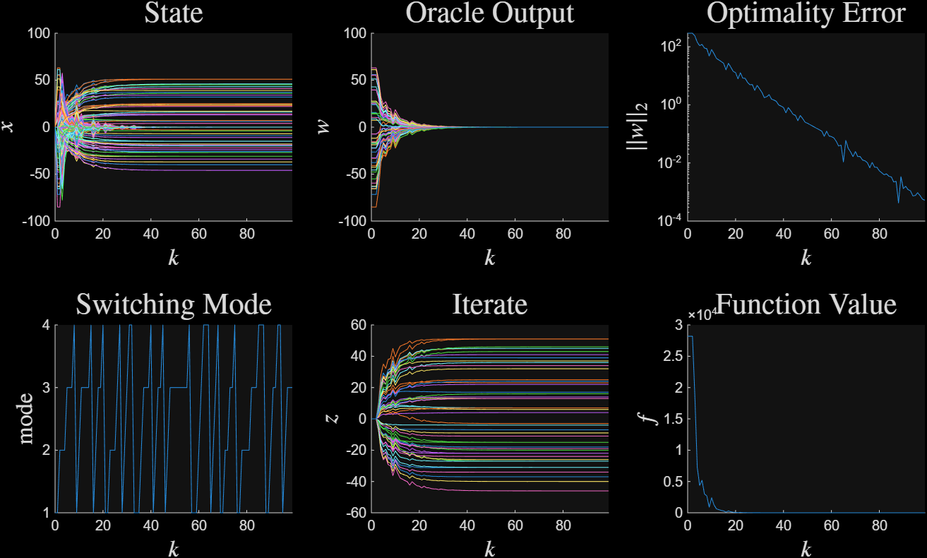
Figure 1: Trace of algorithm simulation convergence

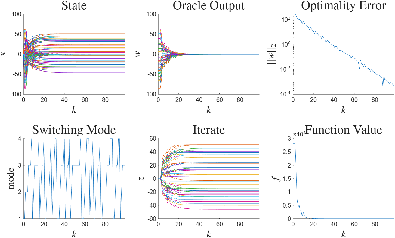
Figure 1: Trace of algorithm simulation and convergence

Figure 2 plots the tracking error over this simulation.

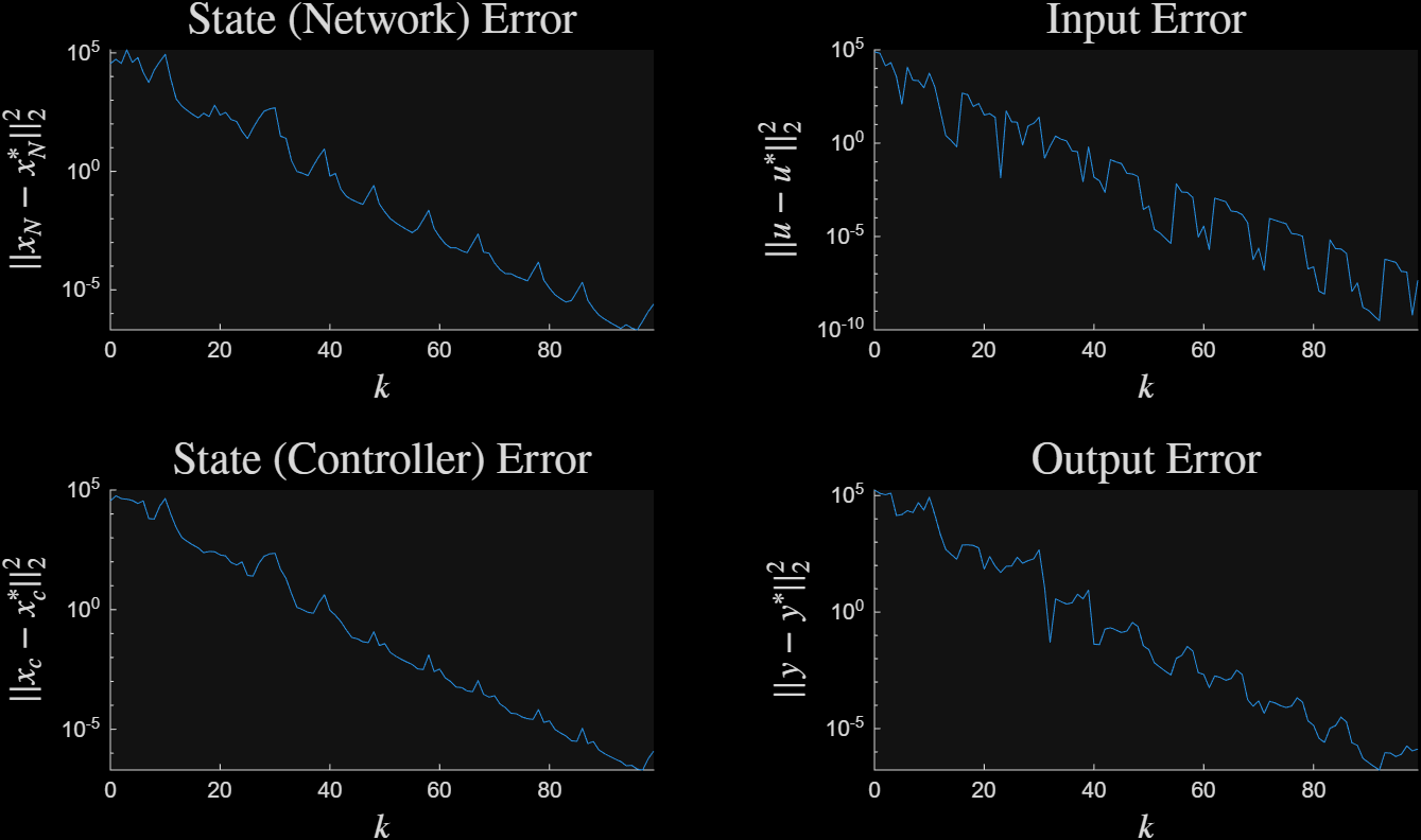
Figure 2: Trace of tracking error

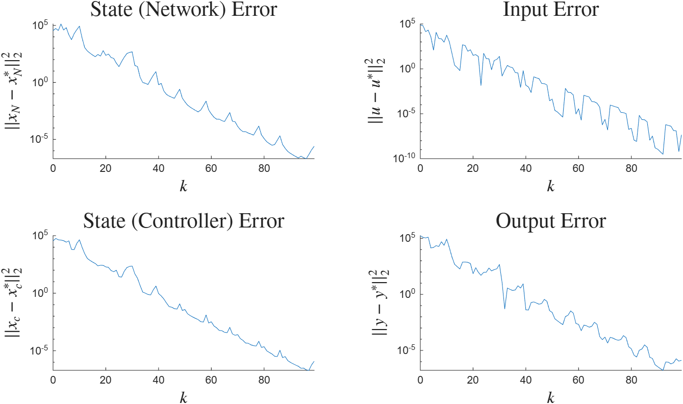
Figure 2: Trace of tracking error

Periodicity can be enforced in two ways. The first is by imposing a periodic switching structure in the adjacency graph as in opt_system_switched.adj = circshift(4, -1). The second method is to use opt_system_periodic instead of opt_system_switched. With the subsystems and function classes in this example, the \(\rho\) bound for the first method is \(0.8212\), while the \(\rho\) bound for the second method is \(0.7028\). This gap is present because the LMIs in the general switched system program are more conservative than the LMIs for the more targeted periodic system program.

Code for ring-switched synthesis at \(m=1, L=2\)

%generate the state space subsystems
P =cell(4, 1);
nx = 2;
P{1} = [0 , 0 , 1 , 0;
    0 , 0.2 , 0 , 1; 
    0 , 1 , 0 , 0 ; 
    -1 , 0 , 0 , 0];

P{2} = [0.2 , 0 , 0.25 , 0;
    0 , 0.9 , 0 , 1 ; 
    0 , 1 , 0 , 0 ; 
    -0.4 , 0 , -0.5 , 3];

P{3} = [-0.3 , 0 , 0.5 , 0;
    0 , -0.5 , 0 , 1 ;
    0 , 1 , 0 , 0 ; 
    -0.3 , 0 , 0.5 , 1];

P{4} = [1.2 , 0 , 1 , 0;
    0 , -0.2 , 0 , 1 ;
    0 , 1 , 0 , 0 ;
    1 , 0 , 0 , 2];

%break up the subsystems into genplants
Plist = cell(4, 1);
n = struct('nw', 1, 'nz', 1, 'ny', 1, 'nu', 1);
for i = 1:4
    A = P{i}(1:nx, 1:nx);
    B = P{i}(1:nx, (nx+1) : end);
    C = P{i}((nx+1) : end, 1:nx);
    D = P{i}((nx+1) : end, (nx+1) : end);
    Plist{i} = genplant(ss(A, B, C, D, 1), n);
end

network = genplant_poly(Plist);


%ring switching transition graph
Gring = [1, 1, 0, 0;
         0, 1, 1, 0;
         0, 0, 1, 1;
         1, 0, 0, 1];


%define the operator
m = 1; L = 2;
ops = {op_sml(m, L)};

sys = opt_system_switched(ops, network, [], Gring);

%only allow gradients
config =opt_config();
config.syn.prox = 0;

%pose and solve
man= opt_synthesis(sys, config);