Tracking an Oscillator

This example continues the Oscillator simulation demonstration.

Figure 1 plots bounds on the convergence rate \(\rho\) as \(\omega\) is swept in the range \([-\pi, \pi]\). Each Analysis run uses the same orders for each operator. The \(\rho=1\) stability boundary is shown by the gray dashed line, convergence is certified if \(\rho <1\).

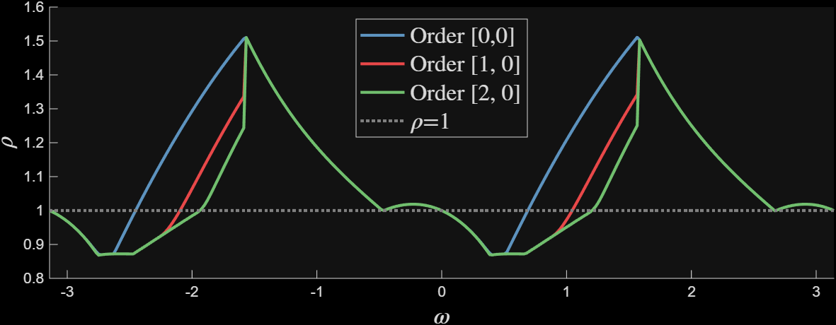
Figure 1: Convergence rate bound v.s. \(\omega\)

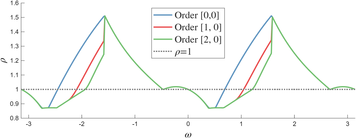
Figure 1: Convergence rate bound v.s. \(\omega\)

Figure 1 certifies algorithm convergence at \(\pi/4 \approx 0.7854\), and does not certify convergence at \(\pi/2\approx 1.5708\). Figure 2 plots an algorithm trajectory at the certified-convergent \(\omega = \pi/4\).

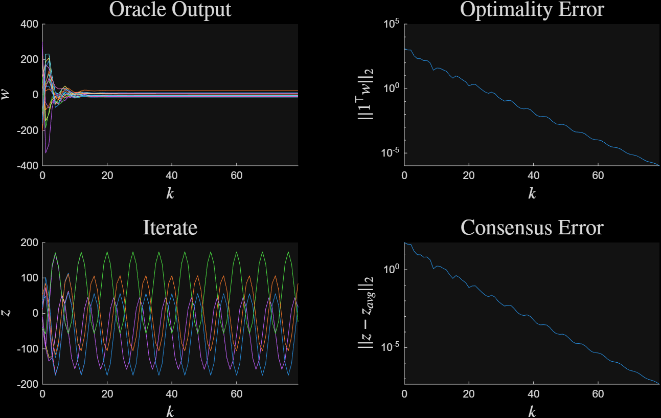
Figure 2: Convergence at \(\omega = \pi/4\)

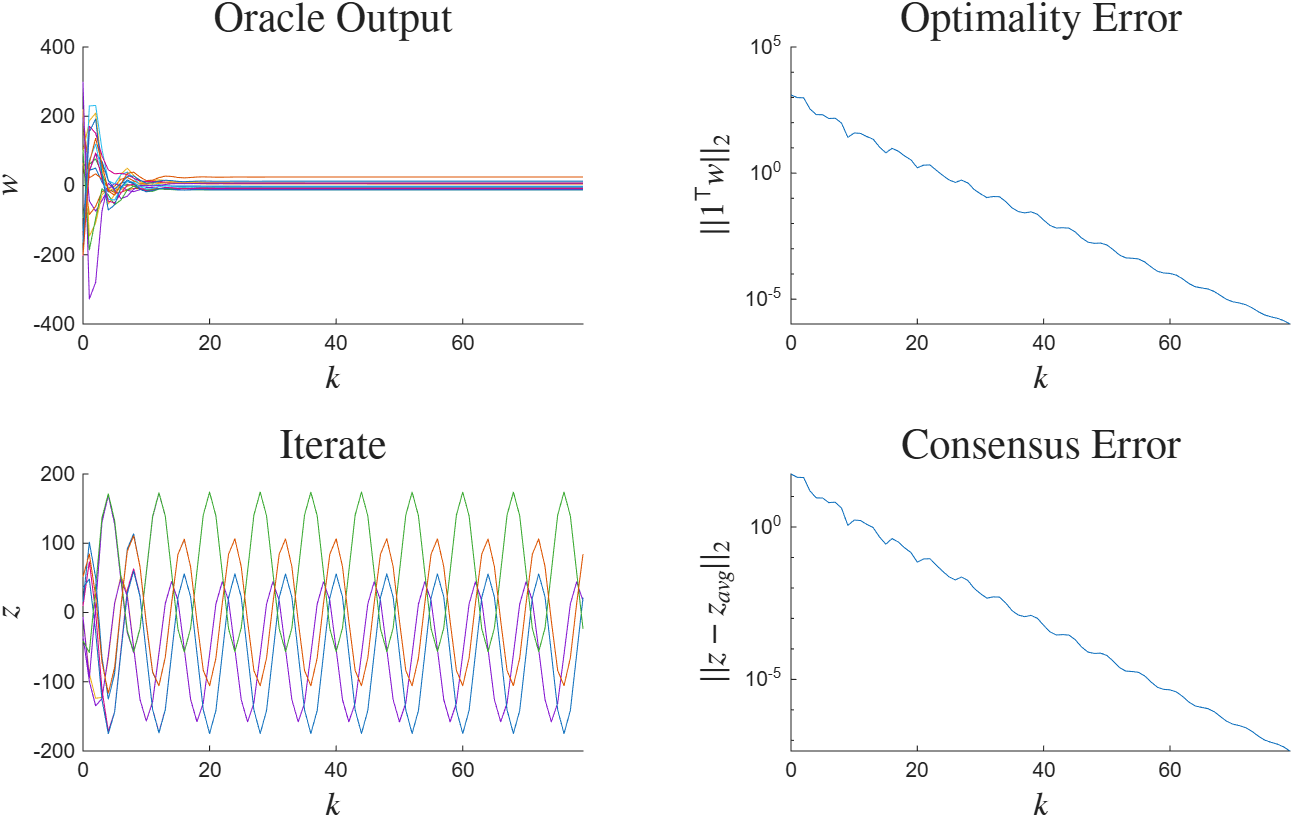
Figure 2: Convergence at \(\omega = \pi/4\)

Figure 3 plots a nonconvergent algorithm trajectory at \(\omega = \pi/2\).

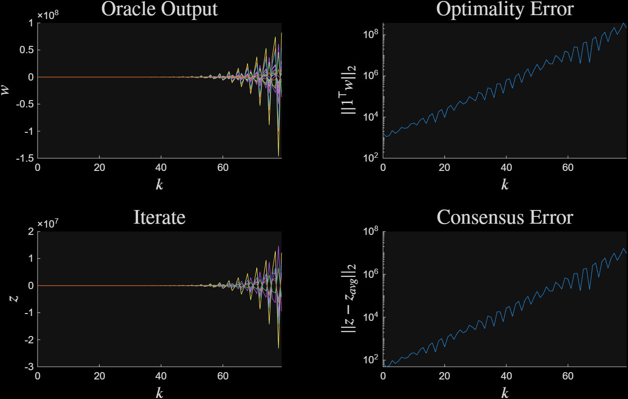
Figure 3: Nonconvergence at \(\omega = \pi/2\)

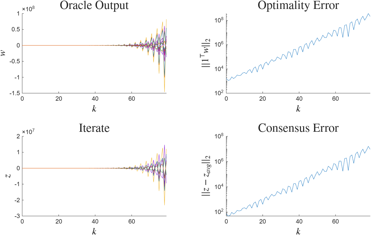
Figure 3: Nonconvergence at \(\omega = \pi/2\)

Code for Oscillator Tracker Analysis at order [2, 0], sweeping over \(\omega\)

%define the operators
m = [1, 1, 1, 1];
L = [2, 4, 6, 8];
s = length(m);

op_list = cell(s, 1);
for i = 1:s
    op_list{i}= op_sml(m(i), L(i));       
end

%parameters of the controller, independent of omega
b0 = [-0.05; -0.1; -0.05];
b1 = -0.05;
b2 = -0.1;

BK = b0 * ones(1, s);
CK = ones(s, 1) * Rbeta;

DK = zeros(s);
DK(end, :)= DK(end, :) + b1;
DK(:, 1)= DK(:, 1) + b2;


%sweep over the angle
Nomega = 320;
omegalist = pi * linspace(-1, 1, Nomega);

rholist = zeros(1, Nomega);

order = {2, 2, 2, 2};
parfor i = 1:length(omegalist)

    %define the path of the optimal solution
    theta = omegalist(i);
    Sbeta = blkdiag(1, givens(cos(theta), sin(theta)));
    Rbeta = [1, 1, 0];

    
    %create the controller    
    K = ss(Sbeta, BK, CK, DK, 1);
    
    
    %form the system
    sys = opt_system(op_list, [], K);
    
    
    %run Analysis and store result
    man = opt_analysis(sys);  
    sol = man.bisect(order);

    rholist(i) = sol.rho;    
end