

Noisy Douglas Rachford#
The Douglas-Rachford algorithm is a procedure for solving a two-operator inclusion problem [1]. It is characterized by parameters \(\gamma, \lambda > 0\), and can be described as the interconnection
The Douglas-Rachford algorithm is used in this example to solve a composite optimization problem
The necessary optimality condition for this problem is posed using the operators \(F_1 = \partial f\), and \(F_2 = \partial \mathbb{I}_{\norm{\cdot}_\infty \leq 10}\)
No Noise#
The Douglas-Rachford scheme with parameters \(\gamma = 0.4, \lambda = 1\) is executed for a problem where \(f\) is a convex quadratic (eigenvalue bounds \(m = 1, L = 10\)). Figure 1 plots a trajectory of Douglas-Rachford starting from \(x_0 = 0\).
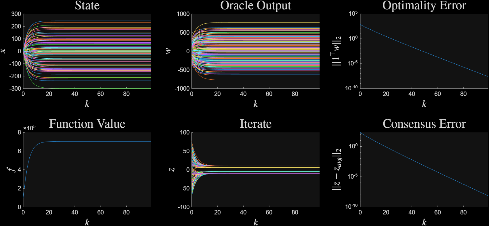
Figure 1: Convergence without noise#
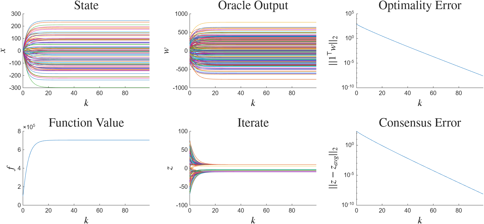
Figure 1: Convergence without noise#
With Noise#
Noise is then added to the Douglas-Rachford execution. The performance input \(w_p\) introduces additive noise at the output of the subgradient evaluations. The performance output \(z_p\) is the consensus error \(\pm \frac{1}{2}(z_1 - z_2)\). The System representing Douglas-Rachford with this noise structure is
Figure 2 plots a trace of a trajectory starting at \(x_0=0\), in which the performance input \(w_p\) is randomly sampled subject to the bound \(\norm{w_{p,k}}_2 \leq 10, \forall k \in \N\).
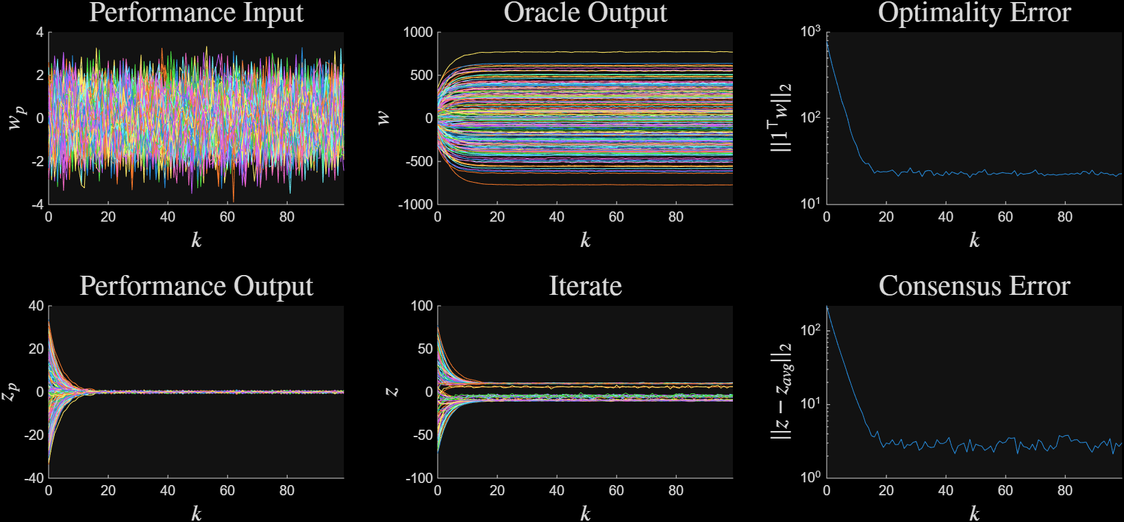
Figure 2: Response under bounded noise#
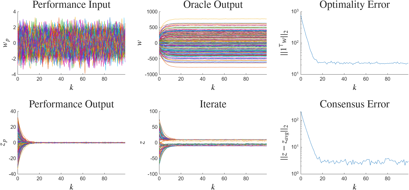
Figure 2: Response under bounded noise#
 1%Douglas Rachford Algorithm with noise
 2rng(32, 'twister');
 3
 4
 5d = 100; %dimension of variable beta
 6s = 2; %number of operators
 7
 8%define the quadratic
 9m = 1; L = 10;
10Q = rand_quad(d, m, L);
11zstar = 100*(2*rand(d, 1) - 1);
12op1 = op_sim_quad(Q, zstar);
13
14%define the L infinity ball
15BOX = 10;
16op2 = op_sim_box(BOX);
17ops = {op1, op2};
18
19%douglas-rachford
20gamma = 0.4;  lambda = 1;   %stepsizes
21K = ss(1, [-gamma*lambda, -gamma*lambda], [1; 1], [-gamma, 0; -2*gamma, -gamma],1);
22
23%create the network
24network = bridge_pass_through(s);
25%add noise to the subgradients (outputs of oracles)
26iwp = [1,2];
27izp = [];
28network = network.add_oracle_input(iwp, izp);
29
30%consensus error as a performance condition
31network  = network.perf_output_con();
32
33%form the system
34sys = opt_system(ops, network, K);
35sys_clean = opt_system(ops, [], K);
36
37%% simulate and plot
38T = 100;
39
40%no noise
41sim_clean = alg_sim(sys_clean, d);
42sim_out_clean = sim_clean.sim(T);
43plt_clean = alg_plotter(sim_out_clean);
44fig_clean = plt_clean.plot({'x', 'w', 'res_w', 'f', 'z', 'res_z'},  2);
45
46%with noise
47sim = alg_sim(sys, d);
48
49eps_w = 10; %norm(w_k, 2) <= eps_w at each k
50sim.sampler.wp = @(param)  eps_w * (ball_sample(length(iwp), d));
51
52sim_out = sim.sim(T);
53plt_noisy = alg_plotter(sim_out);
54fig_noisy = plt_noisy.plot({'wp','w', 'res_w', 'zp','z',  'res_z'},  3);