

Cocoercive plus Strongly Monotone#
This example involves finding the solution to a two-operator inclusion problem, where \(F_1\) is \(\beta\)-cocoercive and \(F_1\) is \(\mu\)-strongly maximal monotone. The Douglas-Rachford Algorithm with parameters \(\lambda = 1, \gamma = 1\) is used to solve this problem,
The explicit minimal rate \(\rho\) for this Douglas Rachford algorithm is (Corollary 4.2[1])
Analysis is performed to numerically estimate this minimal rate at order {1, 1}. The parameter \(\mu\) is fixed to 1, and \(\beta\) is swept from \(\beta \in [10^{-2}, 10^2]\). Figure 1 plots the computed and true contraction rates on top, and the error in the estimates on the bottom.
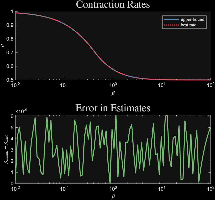
Figure 1: Estimates of the Douglas Rachford Convergence Rate#
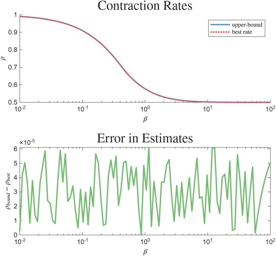
Figure 1: Estimates of the Douglas Rachford Convergence Rate#
Noise is then introduced into the Douglas Rachford execution. The performance input \(w_p\) introduces a shift at the input of each oracle \(F_i\). The performance output \(z\) is the optimality error \(z_{p, k} := w^1_k + w^2_k\). Figure 2 plots the \(\ell_2\) gain between \(w_p\) and \(z_p\) as a function of the cocoercivity parameter. The gain rises as the cocoercivity parameter decreases.
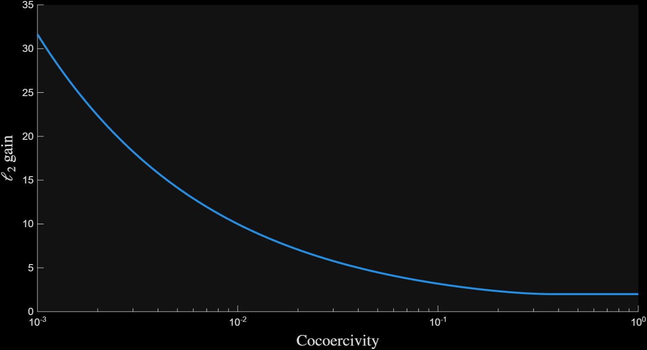
Figure 2: Gain of Douglas Rachford#
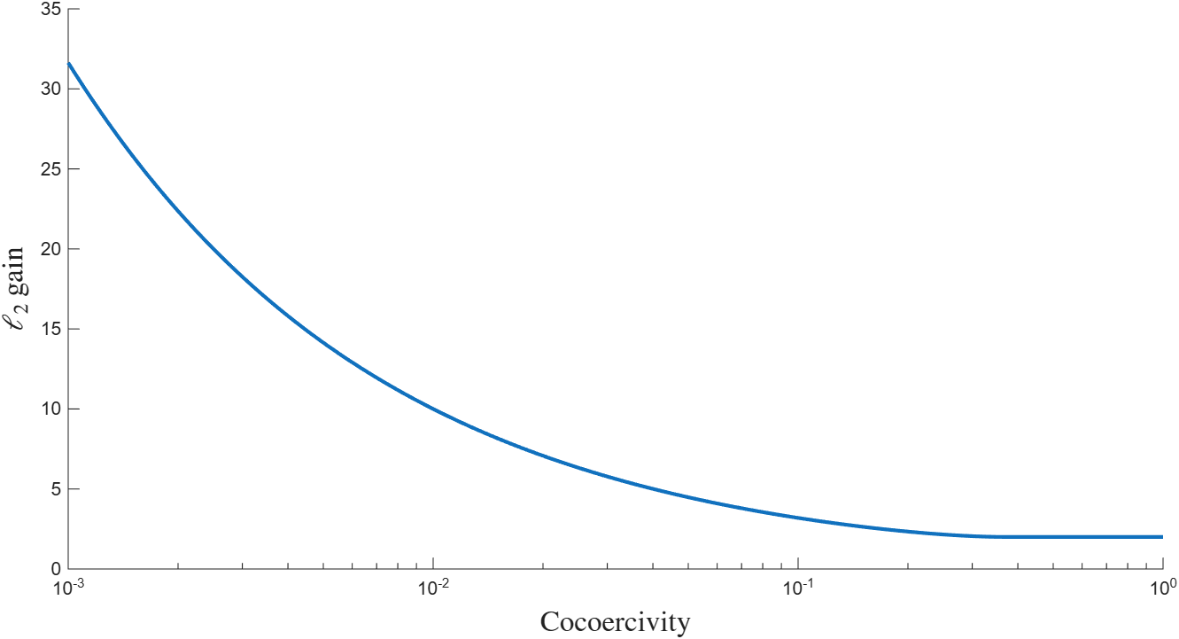
Figure 2: Gain of Douglas Rachford#
 1%cocoercive plus strongly monotone
 2mu = 1; beta = 1.5;
 3
 4%sweep beta
 5Nbeta = 100;
 6beta_sweep = logspace(-2, 2, Nbeta);
 7
 8%description of operators
 9op1 = op_gen();
10op1.monotone = mu;
11
12op2 = op_gen();
13
14%douglas rachford
15gamma = 1; lambda = 1;
16
17K = ss([1],    [-lambda*gamma, -lambda*gamma], ...
18       [1; 1], [-gamma, 0;  -2*gamma, -gamma], 1);
19
20%form the system
21sys = opt_system({op1, op2}, [], K);
22
23%solve the problem
24order = {1, 1};
25man = opt_analysis(sys);
26
27rho_best_dr = zeros(Nbeta, 1);
28rho = zeros(Nbeta, 1);
29%set and solve
30for i = 1:Nbeta
31    %assign the sweep
32    man.sys.op{2}.cocoercive = beta_sweep(i);
33
34    %compute bound
35    sol = man.bisect(order);
36    rho(i) = sol.rho;
37
38    %find the true rate
39    rho_best_dr(i) = best_dr_rate(mu, beta_sweep(i));
40end
This example was inspired by the demonstration in AutoLyap.