Repeated Evaluations

This example performs simulation of the the Bind. The algorithm with parameters \(\lambda, \gamma > 0\) is used to solve a three-operator inclusion problem.

\[\begin{split}\mat{c}{x_{k+1} \hl z^1_k \\ z^2_k \\ z^3_k \\ z^4_k} &= \mat{c|cccc}{I & -2\gamma \lambda I & -\gamma \lambda I& -2\gamma \lambda I & -\gamma \lambda I \hl I & -\lambda I & 0 & 0 & 0 \\ I & -\lambda I & 0 & 0 & 0 \\ I & -2\lambda I & -\lambda I & -\lambda I & 0 \\ I & -2 \lambda I & -\lambda I & - \lambda I & 0} \mat{c}{x_k \hl w^1_k \\ w^2_k \\ w^3_k \\ w^4_k}, \quad & \mat{c}{w^1_k \\ w^2_k \\ w^3_k \\ w^4_k} &= \mat{c}{F_1 (z^1_k) \\ F_2 (z^2_k)\\ F_3 (z^3_k) \\ F_2(z^4_k)}\end{split}\]

Operator \(F_2\) is evaluated twice per iteration, at instants 2 and 4. In this simulation, the operators \(F_1\) and \(F_2\) are gradients of quadratics, and \(F_3\) is the subdifferential of an \(L_\infty\) norm indicator function.

Figure 1 plots an algorithm execution with \(\gamma = 0.4, \lambda = 0.25\) starting from a random initial state \(x_0\), for a problem with variable \(\beta \in \R^{200}\).

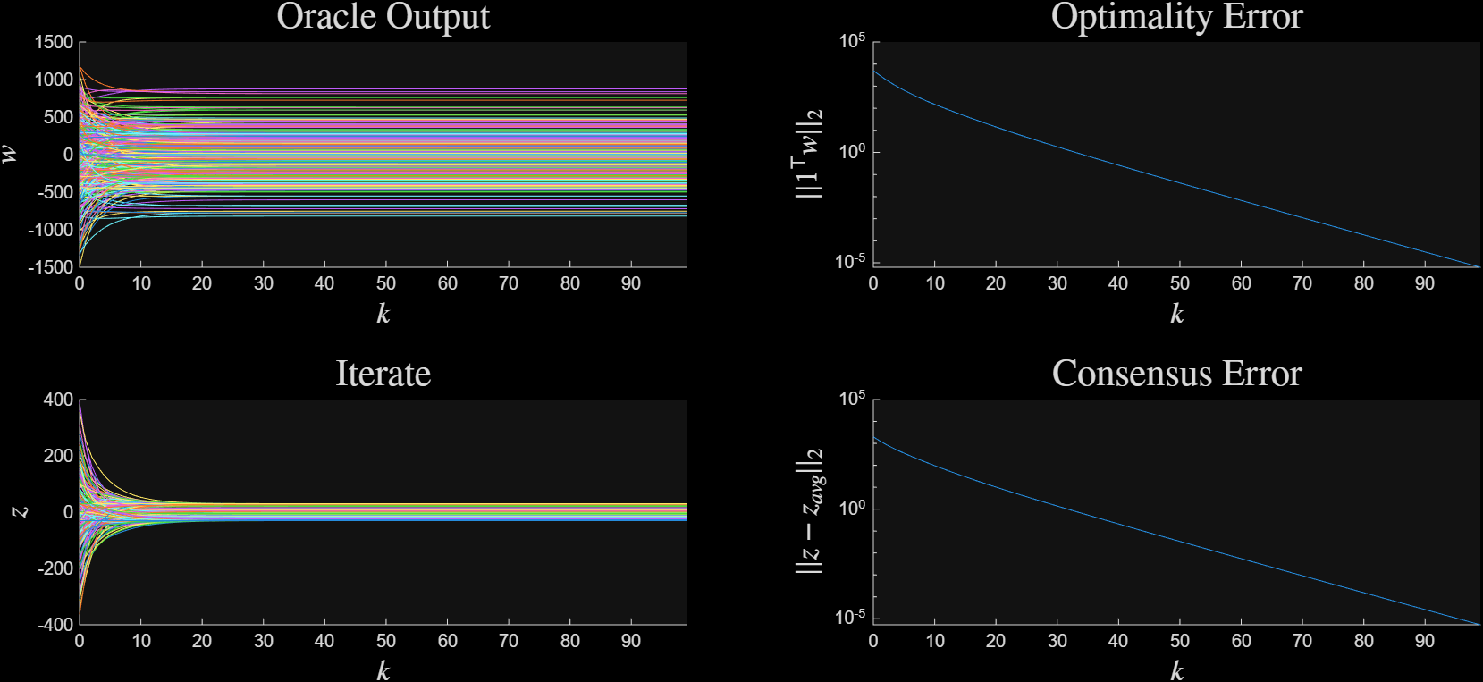
Figure 1: Algorithm with bind \([1, 2, 3, 2]\)

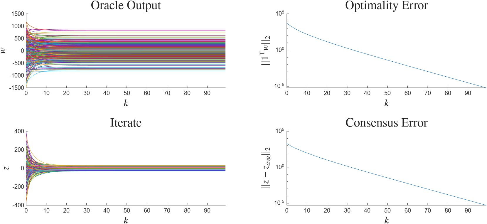
Figure 1: Algorithm with bind \([1, 2, 3, 2]\)

Code for optimization with repeated operator evaluation

%simulation of a multi-step algorithm
rng(40, 'twister');
d = 200; %dimension of problem



%% create a multi-step controller that satisfies the regulator equation
gamma = 0.4;    %stepsizes
lambda = 0.25;


A = 1;
B = -gamma*lambda * [2, 1, 2, 1];
C = ones(4, 1);
D = -lambda * [1, 0, 0, 0;
               1, 0, 0, 0;
               2, 1, 1, 0;
               2, 1, 1, 0];


K = ss(A, B, C, D, 1);


%% form the operators


%randomly generate the quadratics
m1 = 1; m2 = 0;
L1 = 3; L2 = 6;
Q1 = rand_quad(d, m1, L1); bstar1 = randn(d, 1)*100 - 20;
Q2 = rand_quad(d, m2, L2); bstar2 = randn(d, 1)*100 + 20;

BOX = 30; %L infinity norm constraint

%create the operators
op1 = op_sim_quad(Q1, bstar1);
op2 = op_sim_quad(Q2, bstar2);
op3 = op_sim_box(BOX);
ops = {op1, op2, op3};

%put the system together
bind = [1, 2, 3, 2]; %assign the ordering of operators
sys = opt_system(ops, [], K, bind);

%% simulate and plot
sim = alg_sim(sys, d);
% T = 200;
T = 100;
sim.sampler.x0 = 200*randn(1, d);
sim_out= sim.sim(T);
plt = alg_plotter(sim_out);
fig1 = plt.plot_4(1);

zend = sim_out.z(:, :, end);