

Nash Equilibrium Seeking#
This example involves finding a variational Nash Equilibrium of a Linear-Quadratic game. Four agents are interacting in a noncooperative manner. The individual agent decisions are each described in a vector \(\beta_v \in \R^{5}\) for \(v \in \{1, \ldots, 4\}\). These decisions are concatenated into a vector \(\beta \in \R^{20}\).
Each agent is trying to minimize their own quadratic cost
The pseudogradient operator of this game is
The agent strategies are restricted such that \(\norm{\beta}_{\infty} \leq 10\). The point \(\beta^*\) is a variational Nash Equilibrium if it satisfies the variational inequality [1]
Under this condition, no agent \(v\) will unilaterally change their decision \(\beta_v\) to decrease their individual objective. The variational inequality can be converted to an inclusion problem with \(F_2 = \partial \mathbb{I}_{\norm{\cdot}_\infty \leq 10}\)
In this example, the affine pseudogradient operator \(F_1\) has strong monotonicity constant \(\mu = 1.4785\) and cocoercivity constant \(\beta = 0.1605\). This game therefore has a unique variational Nash Equilibrium \(\beta^*\).
The Douglas Rachford algorithm with parameters \(\gamma = 1, \lambda =1\) is used to find \(\beta^*\). Figure 1 plots algorithm trajectories starting from the initial condition \(x_0 = 0\). The bottom-left plot displays the payoffs \(\{f_v(\beta_k)\}_{v =1}^4\) of the individual agents.
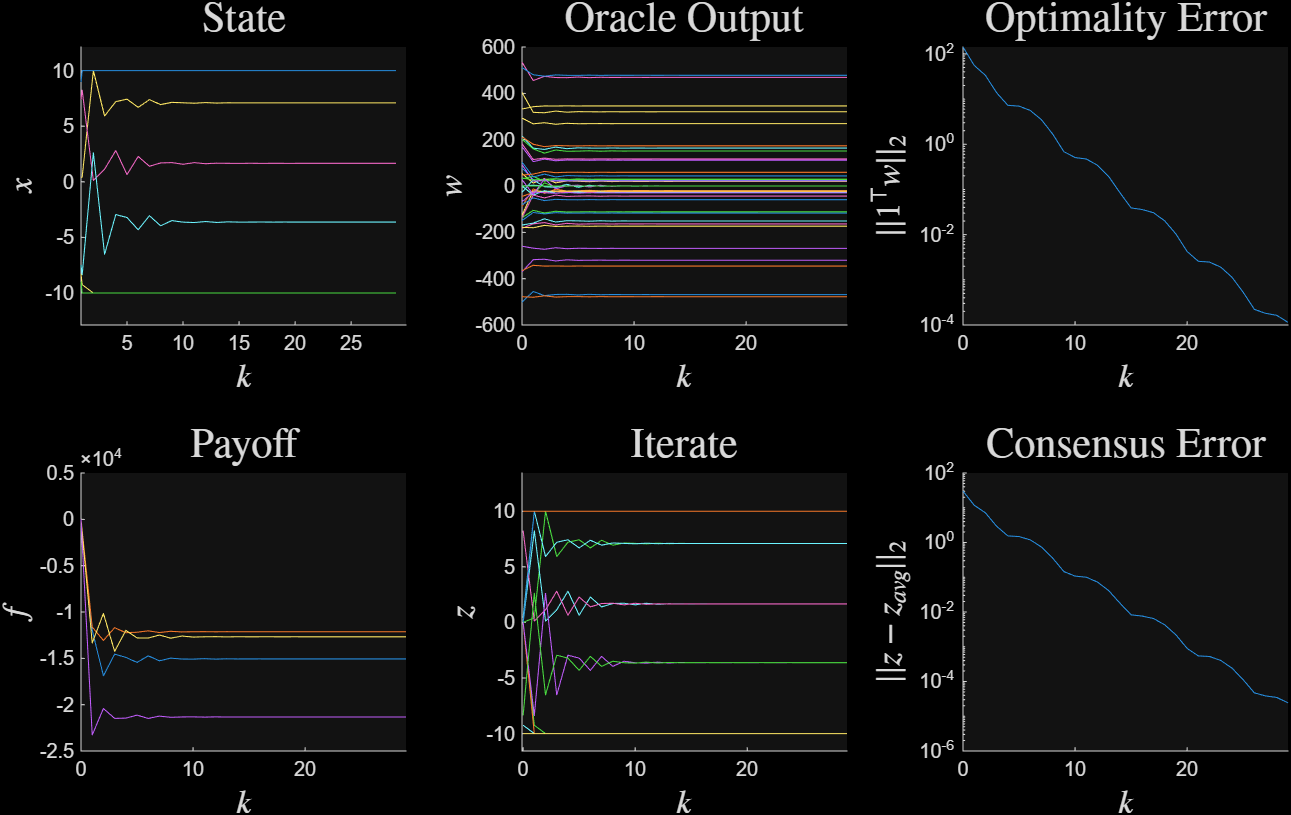
Figure 1: Convergence to the variational Nash Equlibrium#
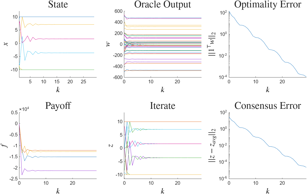
Figure 1: Convergence to the variational Nash Equlibrium#
 1rng(33, 'twister');
 2
 3%define the  game
 4%each agent minimizes a quadratic cost
 5N_agent = 4; %number of agents
 6n = 5*ones(N_agent, 1); %strategy space of each agent
 7mu_boost = 5; %add strong monotonicity
 8[Q_list, b_list, c_list] = rand_LQ_game(n, mu_boost);
 9op1 = op_sim_LQ_game(Q_list, b_list, c_list, n);
10
11
12%define the L infinity ball
13%individual constraints for agents
14BOX = 10;
15op2 = op_sim_box(BOX);
16% op2 = op_sim_l1_hard(BOX);
17ops = {op1, op2};
18
19%douglas-rachford
20gamma = 1;
21lambda = 1;
22
23K = ss([1], [-lambda*gamma, -lambda*gamma], ...
24    [1; 1], [-gamma, 0; -2*gamma, -gamma],1);
25
26%form the system
27sys = opt_system(ops, [], K);
28
29%% simulate and plot
30d = sum(n);
31sim = alg_sim(sys, d);
32T = 100;
33% sim.sampler.x0 = 200*randn(1, d);
34sim_out= sim.sim(T);
35plt = alg_plotter(sim_out);
36plt.plot({'x', 'w', 'res_w', 'payoff', 'z', 'res_z'}, 1);