Tracking an Oscillator#

This example involves a time-varying optimization algorithm (from Tracking). The optimal solution \(\{\beta^*_k\}\) orbits about a constant point \(\beta^*_{\text{center}}\) with a frequency of \(\omega = \frac{\pi}{8}\) radians per time step.

The optimization problem is to minimize the sum of four quadratics. Each quadratic \(f_{ik}\) shares the same shift,

\[f_{ik}(\beta_k - \beta^*_k) = f_{i0}(\beta_0 - \beta_0) \qquad \qquad \forall k \in \N.\]

The path of the optimal solution obeys known linear dynamics: there exists a state \(\eta\) such that

\[\begin{split}\mat{c}{\eta_{k+1} \hl \beta^*_k } = \mat{ccc}{I & 0 & 0 \\ 0 & \cos(\omega) I & -\sin(\omega) I \\ 0 & \sin(\omega) I & \cos(\omega) I \hl I & I & 0} \eta_k.\end{split}\]

The algorithm is defined in terms of parameters \(b_0 \in \R^3, b_1 \in \R, b_2 \in \R\). An execution of this algorithm with \(\beta \in \R^{4}\) is plotted in Figure 1.

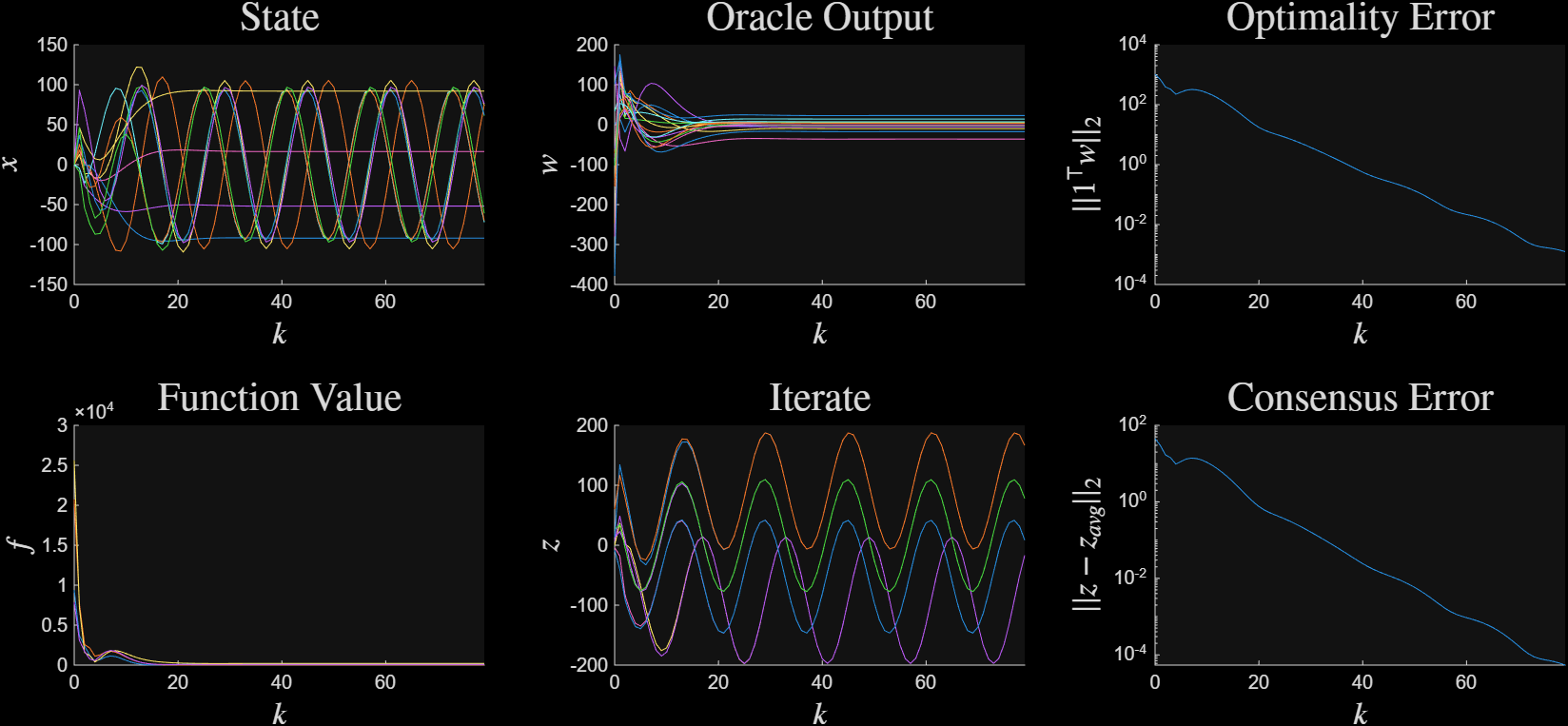
../../_images/track_clean_6_dark.png — *Figure 1:* Algorithm with oscillating target#

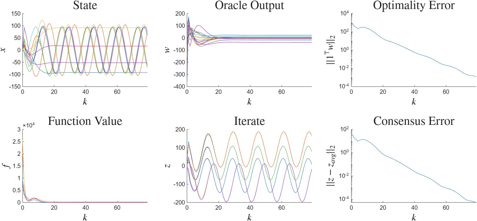
../../_images/track_clean_6_light.png — *Figure 1:* Algorithm with oscillating target#

The subdifferentials \(w\) vectors approach at constant value. The iterates \(z\) oscillate according to the moving optimal solution.

Code for tracking an oscillating target#

%tracking of optimal solution

m = [1, 1, 1, 1];
L = [2, 4, 6, 8];
s = length(m);


omega = pi/8;
Sbeta = blkdiag(1, givens(cos(omega), sin(omega)));
Rbeta = [1, 1, 0];


d = 4; %dimensionality of the problem
%low for illustration


%tracking of the solution
SA = kron(Sbeta, eye(d));
SAy = kron(Rbeta, eye(d));
eta0 = [randi(201, [d, 1]) - 100; 
    (randi(31, [2*d, 1]) + 60).*sign(2*rand(2*d, 1) - 1)];

shift = @(k) SAy * (SA^k) * eta0;

%% assign the quadratics
M = cell(s, 1);
bstar_center = cell(s, 1);
bstar = cell(s, 1);
op_list = cell(s, 1);


for i = 1:s
    M{i} = rand_quad(d, m(i), L(i));
    bstar_center{i} = randi(21, [d, 1]) - 10;    
    bstar{i} = @(k) bstar_center{i} - shift(k);

    op_list{i}= op_sim_quad(M{i}, bstar{i});   
end

%static parameters
b0 = [-0.05; -0.1; -0.05];
b1 = -0.05;
b2 = -0.1;

AK = Sbeta;
BK = b0 * ones(1, s);
CK = ones(s, 1) * Rbeta;

DK = zeros(s);
DK(end, :)= DK(end, :) + b1;
DK(:, 1)= DK(:, 1) + b2;


K = ss(AK, BK, CK, DK, 1);


sys = opt_system(op_list, [], K);

%% execute the algorithm

T = 80;
sim = alg_sim(sys, d);
ssim= sim.sim(T);

%% plot the outputs
plt = alg_plotter(ssim);
plt.plot_6f();