Games with Delay

This example continues the Douglas-Rachford Game simulation demonstration.

In this two-operator example, the pseudogradient \(F_1\) is \(1.4785\)-monotone and \(0.1605\)-cocoercive, and the normal cone \(F_2 = \partial \mathbb{I}_{\norm{\cdot}_{\infty} \leq 10}\) is the subdifferential of a p.c.c. function. The operators are therefore described by op_gen and op_pcc respectively.

Four algorithms to solve this inclusion problem are synthesized.

1. Backward evaluation of both \(F_1\) and \(F_2\),

2. Forward evaluation of \(F_1\), backward evaluation of \(F_2\),

3. A delay of one time step before and after evaluation of \(F_1\).

Synthesis is performed for each case without a warm start (iqc=[]). The certified convergence rates are \(\rho < 0.7163\) for Algorithm 1, \(\rho < 0.8734\) for Algorithm 2, and \(\rho < 0.9430\) for Algorithm 3.

All three are certifiably convergent, but Algorithm 1 has the least worst-case convergence rate. Each Synthesis is accompanied by an algorithm Simulation starting from an initial condition \(x_0=0\), empirically demonstrating this speed of convergence

Figure 1 plots a trajectory of the backward evaluation algorithm.

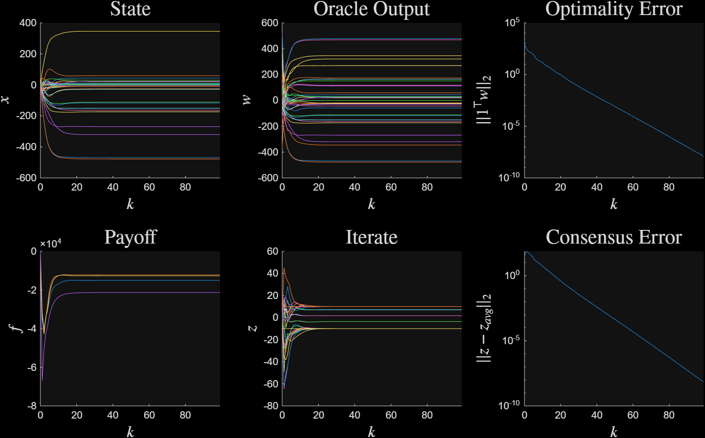
Figure 1: Algorithm with both backward evaluations

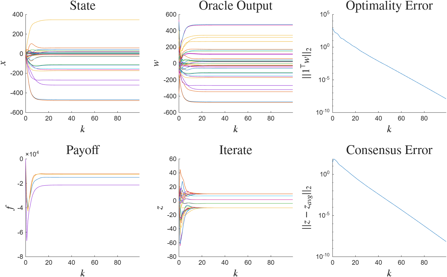
Figure 1: Algorithm with both backward evaluations

Figure 2 plots a trajectory of the forward and backward evaluation algorithm.

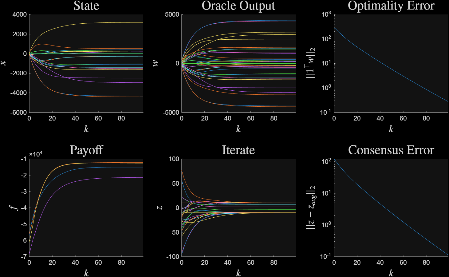
Figure 2: Algorithm with one forward and one backward evaluation

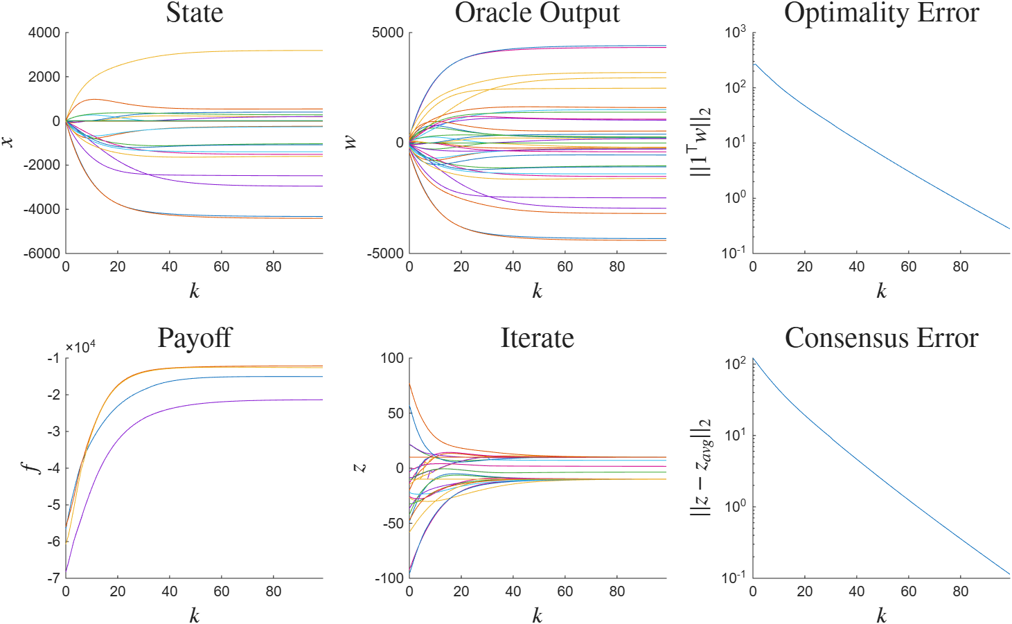
Figure 2: Algorithm with one forward and one backward evaluation

Figure 3 plots a trajectory of the algorithm with time delay.

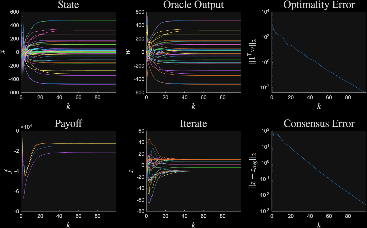
Figure 3: Algorithm with delay on \(F_1\)

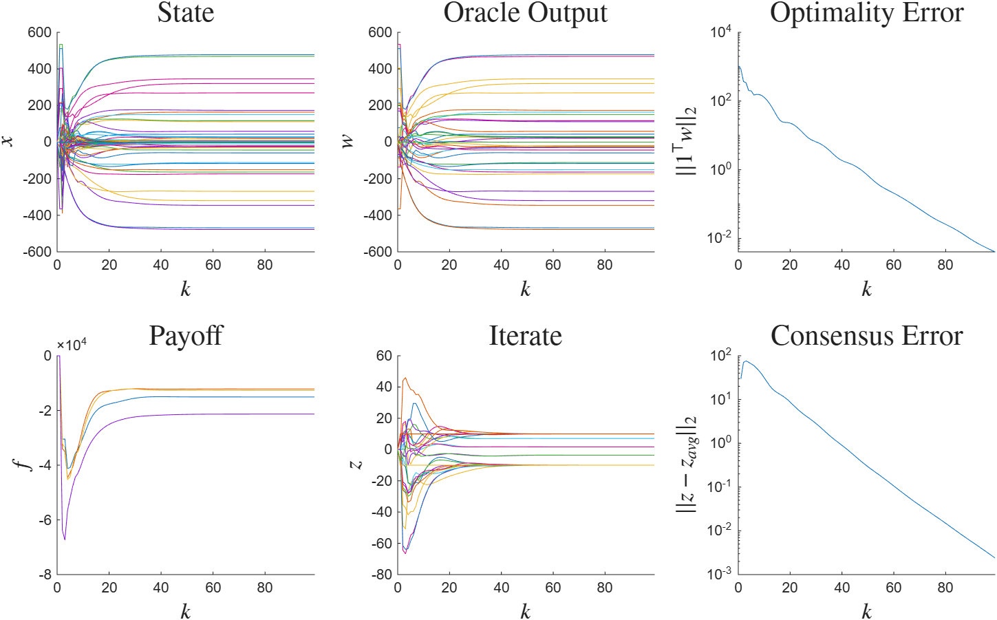
Figure 3: Algorithm with delay on \(F_1\)

Code for Nash Equilibrium Seeking

rng(33, 'twister');

%define the Linear Quadratic Game
N_agent = 4; %number of agents
n = 5*ones(N_agent, 1); %strategy space of each agent
mu_boost = 5; %add strong monotonicity
[Q_list, b_list, c_list] = rand_LQ_game(n, mu_boost);
op1_sim = op_sim_LQ_game(Q_list, b_list, c_list, n);


%% synthesize an algorithm
mu = op1_sim.monotone; %1.4785
beta = op1_sim.coco; %0.1605

op1 = op_gen();
op1.monotone = mu;
op1.cocoercive = beta;

op2 = op_pcc();
ops = {op1, op2};

%form the network delay
d1 = [1, 0];
d2 = [1, 0];
network = bridge_channel_delay(d1, d2);

%form the system
sys = opt_system(ops, [], []);
sys_delay = opt_system(ops, network, []);

%set the information structure
config = opt_config();
% config.syn.elimination = false;

%backward evaluation of pseudogradient
config.syn.D_mask = [1, 0; 1, 1]; 
man_bw = opt_synthesis(sys, config);

%forward evaluation of pseudogradient
config.syn.D_mask = [0, 0; 1, 1]; 
man_fw = opt_synthesis(sys, config);

%delay on pseudogradient, no controller restriction
config.syn.D_mask = [1, 1; 1, 1]; 
man_delay = opt_synthesis(sys_delay, config);

sol_bw = man_bw.bisect();       %rho = 0.7163
sol_fw = man_fw.bisect();       %rho = 0.8734
sol_delay = man_delay.bisect(); %rho = 0.9430

%% simulate and plot

%define the L infinity ball
%individual constraints for agents
BOX = 10;
% op2_sim = op_sim_box(BOX);
op2_sim = op_sim_l1_hard(100);
ops_sim = {op1_sim, op2_sim};

sys_sim_fw = sol_fw.sys.export_sim(ops_sim);
sys_sim_bw = sol_bw.sys.export_sim(ops_sim);
sys_sim_delay = sol_delay.sys.export_sim(ops_sim);


sys_sim_list = {sys_sim_fw, sys_sim_bw, sys_sim_delay};

for i =1:3
    d = sum(n);
    sim = alg_sim(sys_sim_list{i}, d);
    T = 100;
    
    sim_out= sim.sim(T);
    plt = alg_plotter(sim_out);
    plt.plot({'x', 'w', 'res_w', 'payoff', 'z', 'res_z'}, i);
end