Sequential Games

The four-player game is continued from the simulation example. Its pseudogradient map \(F_1\) is affine, \(1.4785\)-monotone and \(0.1605\)-cocoercive.

This example performs Synthesis of a Nash Equilibrium seeking algorithm in two scenarios:

1. Simultaneous: each agent updates its strategy \(z^i_k\) at every time step \(k\)

2. Sequential: the agents take turns updating their strategies, \(z^i_k\) changes only once per four time steps.

Both algorithms permit only explicit evaluations of the pseudogradient map \(F_1\).

The Simultaneous setting involves an LTI system, and returns an algorithm with convergence rate \(\rho \leq 0.8733\). The Sequential setting is modeled as a periodic-orbit system, and yields an algorithm with convergence rate \(\rho \leq 0.9667\).

Figure 1 plots a trajectory of the simultaneous game.

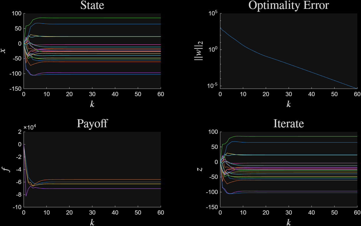
Figure 1: Simultaneous play of the game

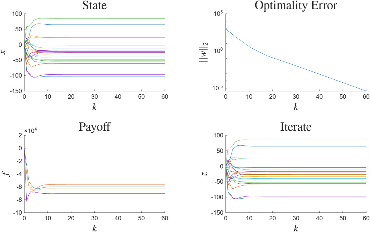
Figure 1: Simultaneous play of the game

Figure 2 plots a trajectory of the sequential game.

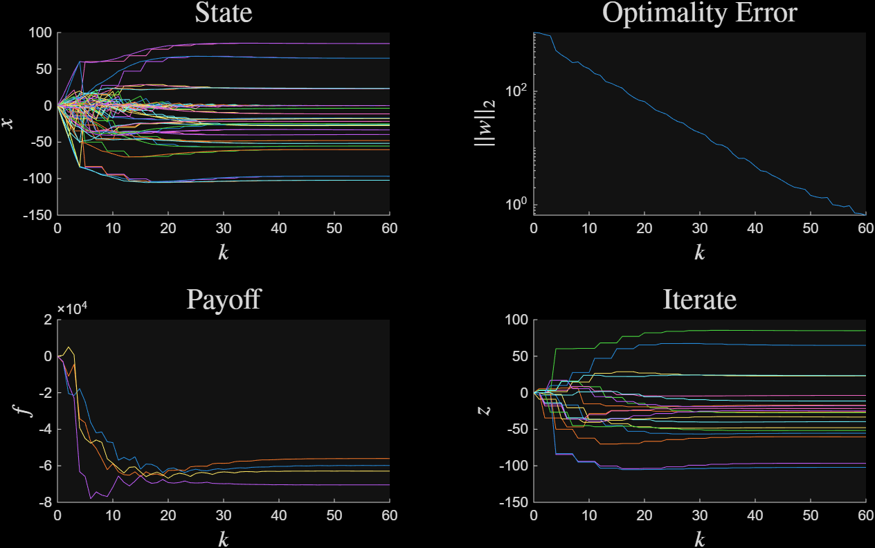
Figure 2: Sequential play of the game

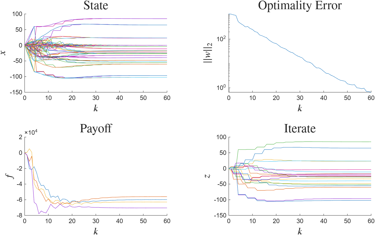
Figure 2: Sequential play of the game

In the designed sequential algorithm, each agent \(i\) has full knowledge of the entire pseudogradient vector \(w_k\). The partial knowledge setting involves allowing only the actively playing agent \(i\) access to \(w^i_k\). Synthesis in this partial knowledge setting returns an infeasible controller \((\rho \geq 2)\).

Code for sequential Nash Equilibrium Seeking

%parameters of the game
mu = 1.4785; beta = 0.1605;
%number of agents

%describe the operators
op1 = op_gen();
op1.monotone = mu;
op1.cocoercive = beta;

ops = {op1};

%form the network
c=4; 
M = circshift(eye(c), -1); %cyclic sequential play
network = coordinate_descent_system(c);

%form the systems
sys_simul = opt_system(ops);
sys_coord = opt_system_periodic_orbit(ops,  network, [], M);

%pose managers
config = opt_config();
config.syn.prox= 0;
man_simul = opt_synthesis(sys_simul, config);
man_coord = opt_synthesis(sys_coord, config);

%solve
sol_simul = man_simul.bisect();
sol_coord = man_coord.bisect();