

LASSO#
This demonstration applies Synthesis towards LASSO [1] solvers. The hard LASSO problem is
The LASSO problem with \(E \in \R^{m \times n}\) is overparameterized if \(n > m\), and is underparameterized if \(n < m\). It is assumed that \(E\) has full row rank.
In the overparameterized regime, the convex least-squares function \(f(\beta) = \frac{1}{2}\norm{Ex - b}_2^2\) is a member of \(S_{0, \sigma_{\max}(E)^2}\). In the underparameterized regime, the strongly convex \(f\) is a member of \(S_{\sigma_{\min}(E)^2, \sigma_{\max}(E)^2}\)
Synthesis of linearly convergent algorithms will take place in the underparameterized regime, and synthesis of ergodically convergent algorithms will occur in the overparameterized regime. These solvers will only implement explicit/forward evaluations of \(f\).
Overparameterized Regime#
A LASSO solver is first Synthesized for an overparameterized system with \(\sigma_{\max}(E)^2 = 138.90\). The first solver performs explicit evaluations of the least squares cost. Ergodic convergence is approximately confirmed with a constraint violation of \(4.68 \times 10^{-12}\). Figure 1 plots a trajectory of this explicit algorithm.
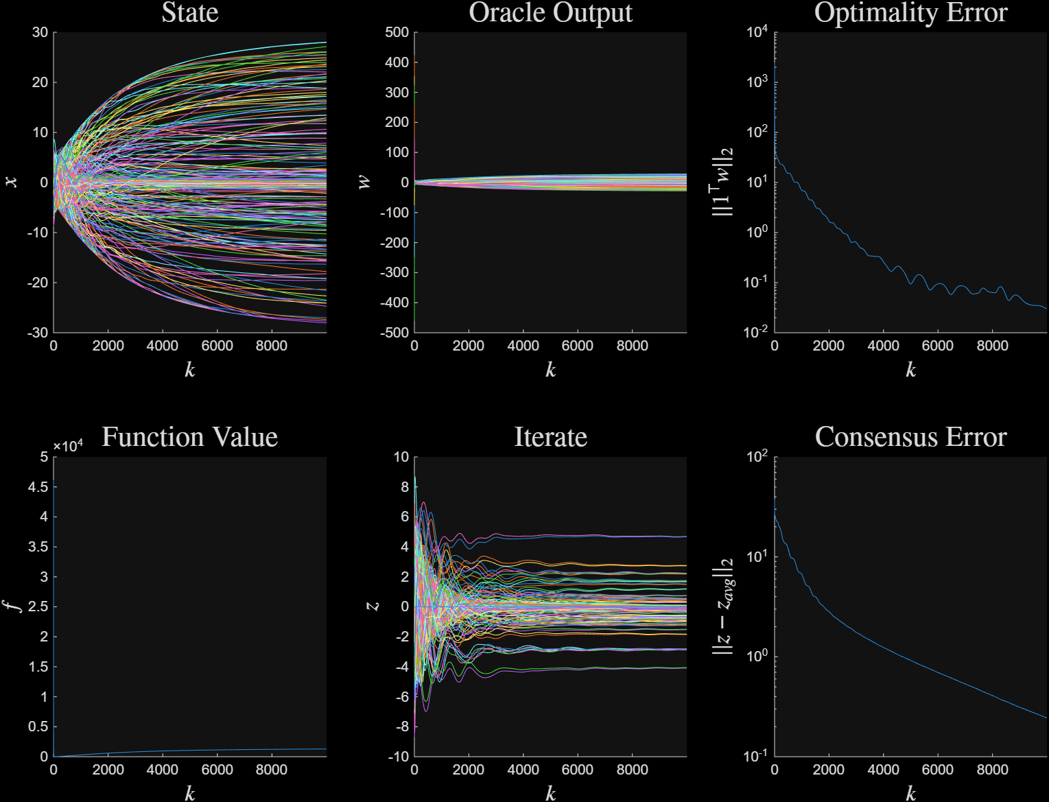
Figure 1: Explicit overparamterized LASSO solution#
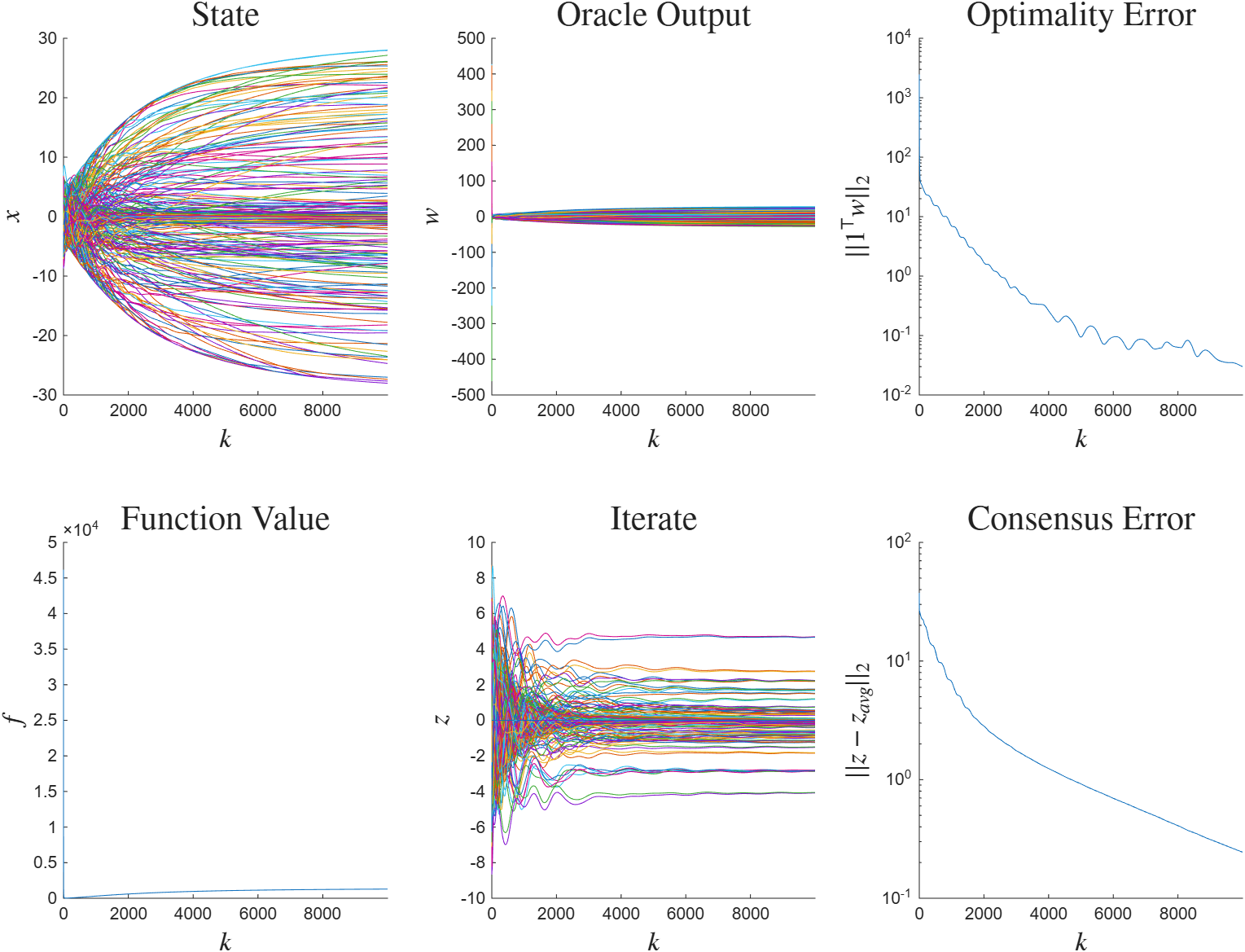
Figure 1: Explicit overparamterized LASSO solution#
% lasso in the underparameterized setting

%% describe the operators
%define the data matrix
rng(430, 'twister');
d = 200;
A_data = 0.5*randn(d/2, d);
b_data = 10*randn(d/2, 1) + 2*rand(d/2, 1);

eK = svd(A_data);
m = 0;
L = max(eK)^2;

op1 = op_sml(m, L);
op2 = op_sml(m, L);
ops = {op1, op2};


%% form the system
sys = opt_system(ops);
spec_erg = spec_ergodic();

%% solve the problem
config =opt_config();
config.syn.D_mask = [0, 0; 1, 1]; %gradient evaluation of lsq

%for sublinear convergence, set lower bounds to the dissipation terms to
%zero (nonstrict dissipation)
config.tol.input_diss = 0;
config.tol.M = 0;
man = opt_synthesis(sys, config);

sol = man.solve_single({}, spec_erg);
Underparameterized Regime#
An explicit algorithm is synthesized for underparameterized setting. The matrix \(E \in \R^{130 \times 100}\) has \(\sigma_{\min}(E)^2 = 2.1933\) and \(\sigma_{\max}(E)^2 = 433.57\). Figure 2 plots an execution of the Synthesized algorithm with linear convergence rate \(\rho \leq 0.99\).
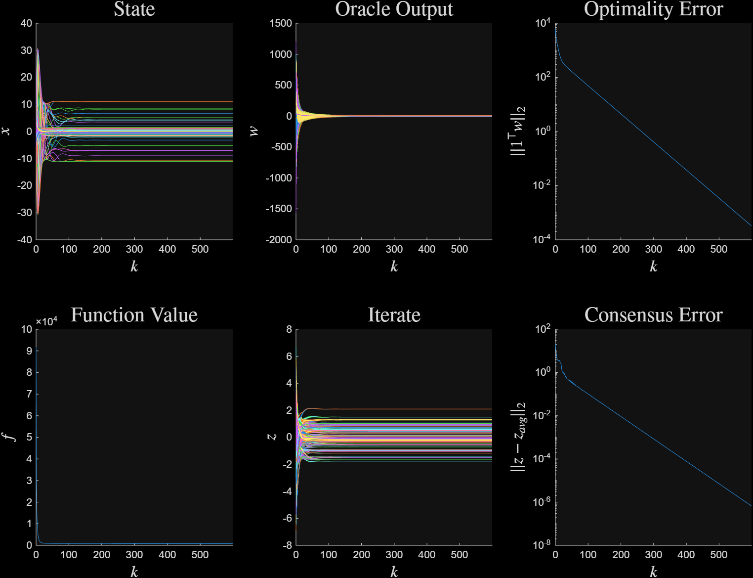
Figure 2: Explicit underparamterized LASSO solution#
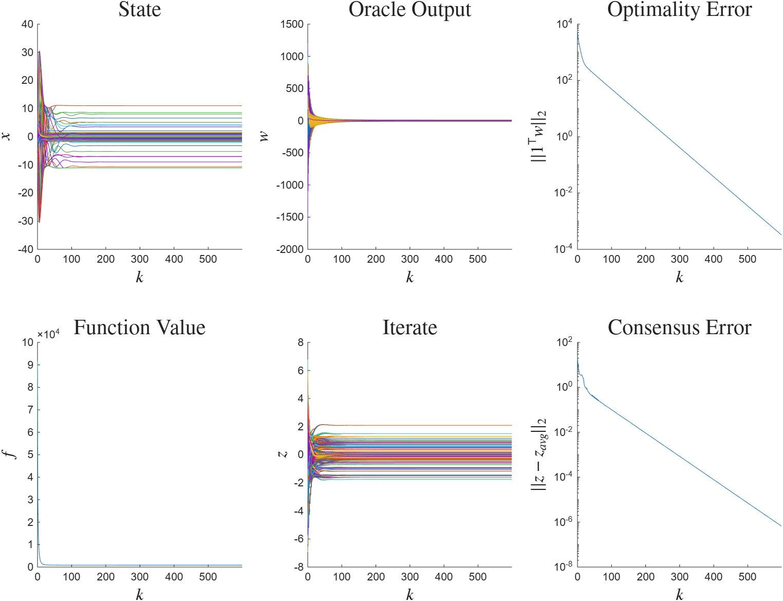
Figure 2: Explicit underparameterized LASSO solution#
%% describe the operators
rng(430, 'twister');

d = 100;
A_data = randn(1.3*d, d);
b_data = 10*rand(1.3*d, 1) + 4*randn(1.3*d, 1);

eK = svd(A_data);
m = min(eK)^2;
L = max(eK)^2;

op1 = op_sml(m, L);
op2 = op_pcc();

ops = {op1, op2};

%% form the system
sys = opt_system(ops);

%% solve the problem
config =opt_config();

%relax stringency of numerical tolerances to encourage a solution

%lowered from default
config.tol.spread = 1e-4;
config.tol.input_diss = 1e-5;
config.tol.M = 1e-9;

%raised from default
config.tol.GX_max = 300;
config.tol.GY_max = 300;
config.syn.elimination_type = 0;
config.syn.D_mask = [0, 0; 1, 1]; %gradient evaluation of lsq
man = opt_synthesis(sys, config);

sol = man.bisect();